An Innovative Way to Predict Continuous Variables: From Regression to Classification

Photo by Tobias Fischer on Unsplash

Introduction: When it comes to the prediction of continuous variables, the first thing that comes to our mind is always the regression model. For instance, linear regression is the most commonly used regression model, and it has the benefits of simple implementation and high interpretability. On the other hand, random forest regression can handle missing data and is adaptive to interactions and nonlinearity. While these algorithms all work well for continuous target variables in different scenarios analytically, they provide less information on the predicted numbers’ confidence level, especially in real-world applications.

In this article, we will explore an unconventional framework to predict continuous variables with given confidence scores. Instead of framing the prediction as a regression problem, we twist the problem into a classification problem. This framework also allows us to have more visibility on the predicted results and can be adjustable to different confidence levels. The article will use revenue estimation as an example. Given a variety of business attributes for many businesses, we will illustrate how we can predict the revenue for each business given a specific confidence level.

From regression to classification

The framework requires more granular data on confidence scores and estimated revenue, and this can be accomplished by transforming the problem into the Binary Relevance (BR) problem. BR involves the decomposition of the target variable into a set of binary classification tasks where each model is learned independently (Madjarov et al., 2012¹).

In real-world applications, it requires dividing the continuous target variable into different thresholds (labels) and training each classification model respectively and independently on one threshold. The revenue thresholds can be set based on specific percentiles of the target continuous variable or certain numbers with special meanings for business use cases. In this revenue estimation example, we are using $1,000, $2,000, $5,000, $10,000 and $20,000 as thresholds and five independent classifiers are trained.

In this case, if one training example is run through the model sets, the output will be five probability scores in accordance with five preset revenue thresholds. For the next step, we want to build a probability curve that indicates the correlation between estimated revenue and confidence scores starting from the five output scores.

Linear interpolation for point estimation

Now that we have five probability scores along with five revenue thresholds, ideally, these five probability scores should be monotonically decreasing considering the distribution of the labels. For instance, if the probability of business revenue greater than $2,000 is 56% based on Classifier 2, considering the class sparsity for different labels and the fact that all classifiers are training on the same data set, the probability predicted from Classifier 1 (greater than $1,000) is expected to be higher based on the class distribution. We will discuss the corner case where the probabilities are not monotonically decreasing later in the article.

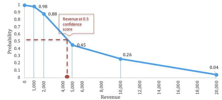
We will also add another threshold Revenue >= $0, then the probability for this threshold is always 1. We plot all five points along with the additional ($0,1) point in the graph. The range of the probability curve that we can obtain is from 1 to the probability of Classifier 5 (Revenue >= $20,000, 0.04), which ideally should be the lower bound. As illustrated in the graph which shows the output of one training example, we can plot the five sets of probabilities and revenues and ($0,1) in a 2d axis and connect the 5+1 points in a linear fashion.

Based on the graph, now we have a probability curve which approximately estimates the correlation between confidence level ranging from the lower bound (0.04) to 1. If a confidence level of 0.5 is the goal, we can obtain the estimated revenue cut off at the 50% confidence score from the curve as is shown on the graph. The estimated revenue at 50% confidence level is the y-axis of the intersection between the horizontal line at 0.5 confidence level and the blue probability curve. This is the point estimation at a 50% confidence level.

Model Performance

For the revenue prediction example, we assess the performance of the classifiers and the accuracy of interpolated revenue. In addition, we also compare the Mean Absolute Error (MAE) of the predicted revenue based on the proposed framework to the MAE of the Random Forest Regression.

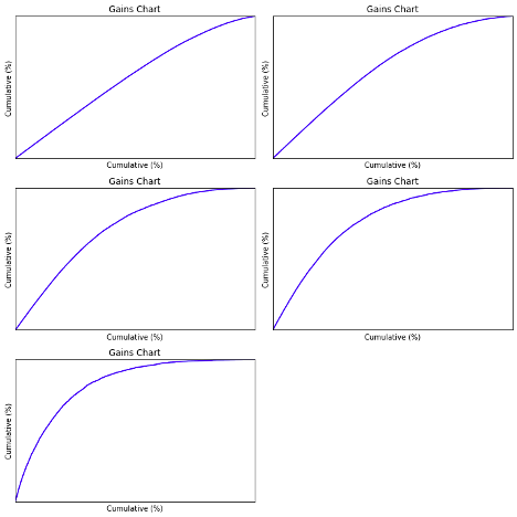
The graphs below demonstrate the gains charts for five classifiers.

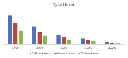
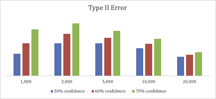
If we use 50%, 60%, and 70% respectively as target confidence level and evaluate the interpolated estimated revenue, for all revenue thresholds the confusion matrices are listed as below. By adjusting the confidence level, we are able to tune the estimated Type I and Type II errors.

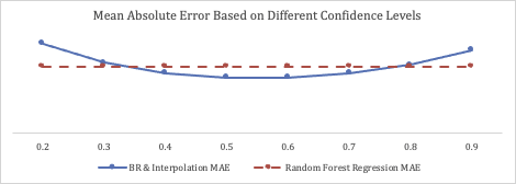
In the chart below, we also compare the Mean Absolute Error (MAE) of two different approaches. The first approach is based on the framework mentioned in this article, and different confidence levels from 0.2 to 0.9 are applied. The second approach is based on Random Forest Regression. The overall MAE for confidence levels from 0.4 to 0.75 is smaller than the MAE of Random Forest Regressor.

Discussion

This framework is proved to work effectively and accurately in business revenue estimation use cases. One of the top advantages of this framework is the capability of adjusting the predicted result for different confidence levels. If a more conservative estimation is expected, we can simply increase the confidence level and vice versa. However, some corner cases need to be handled carefully in this framework.

• The distribution may not be monotonic, depending on the model performance. In an ideal world, if each classifier has significant discriminatory power, we can obtain a monotonic decreasing probability curve based on the class distribution, and only one estimated result is returned for a specific confidence level. In the real world, however, the probability curve may not be monotonically decreasing since we are treating the classifiers independently and ignoring the correlation of the labels. Under this circumstance, more than one estimated result can be returned on some confidence levels. In the revenue prediction use case, since we are more prone to a nonaggressive estimation, the lowest estimation for a confidence level will be the final output. We can also adjust the labels to make the gap between the labels larger to foster a monotonic probability curve.
• There is an upper bound for the estimated revenue output, which is the highest threshold we set, for instance, the $20,000 in the example. The lower bound of the probability curve is always the lowest probability from all classifiers’ output, and it can be very close to zero but not zero exactly, e.g., 0.04 in the graph above. This means we can never have an estimated value in accordance with confidence scores lower than the lower bound of probabilities (0.04). In this use case, the estimated revenue will always be capped at $20,000 since the $20,000 suffices the business needs already.

To serve the purpose of constructing a probability curve, multi-class classification can also be an alternative approach instead of Binary Relevance. BR has the disadvantage of only using the particular label and ignoring the label dependency which leads to the first corner case we mentioned above (Oscar et al., 2012²). However, it also has the following advantages:

• Any binary learner can be applied to train each label, and even of a combination of different binary classifiers training on different labels will work.
• It can be easily parallelized.
• Each classifier has an adequate amount of data to train on since the whole data set is used for each label.
• It optimizes loss function for each label respectively and therefore individual classifier has a satisfactory performance.

We also tested multi-class classification learners in business revenue prediction, but it turned out to underperform the BR approach.

Conclusion

In this article, we provided an unconventional framework to accurately predict a continuous variable and estimate the confidence level of the prediction. We also discussed the application of the framework in business use cases and the limitations of the framework. Even though the framework increases the complexity of the model by converting a conventional one model solution to a multi-model solution, the benefit of visibility into the relationship between confidence levels and predicted values is very valuable. In a fast-changing business environment, the flexibility of tuning confidence levels can be applied to many use cases, which in turn can help with adaptive business decision making in alignment with desired business outcomes.

References

[1] Madjarov, G., Kocev, D., Gjorgjevikj, D., Deroski, S.: An extensive experimental comparison of methods for multi-label learning. Pattern Recognit. 45(9), pp. 3084–3104 (2012)

[2] Oscar Luaces, Jorge Díez, José Barranquero, Juan José del Coz, Antonio Bahamonde: Binary relevance efficacy for multilabel classification (2012)