Solving Dispatch in a Ridesharing Problem Space
Matchings and Graph Theory
The concept of matching drivers to riders can be captured through the lens of graph theory. Thinking of ridesharing matching as a graph comes naturally as the problem inherently involves connecting two distinct groups — riders and drivers. It is also advantageous for several reasons; including the flexibility in modeling relationships (capturing factors like distance, time, and compatibility through weighted edges), as well as offering an armada of efficient and scalable algorithms to identify optimal structures.
One specific graph that captures the ridesharing settings (and more generally any two-sided marketplace setting) is the bipartite graph. Formally, a bipartite graph is a graph where the vertices can be divided into two disjoint sets such that all edges connect a vertex in one set to a vertex in another set. There are no edges between vertices within the same set.
Zoom image will be displayed
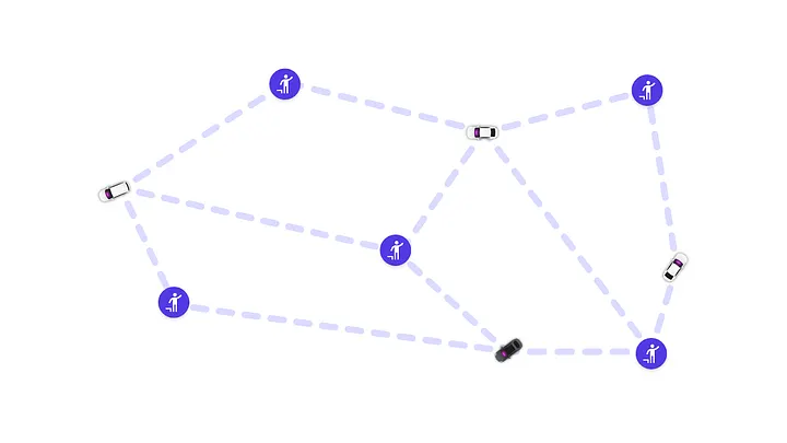
Figure 1: Constructing a bipartite graph to connect drivers to riders
In most cases, our matching graphs are bipartite because we match one rider to one driver. However, there exist more involved situations, like shared rides, where the graph does not satisfy this condition. For simplicity, we only focus on bipartite cases.
Another practical layer that can be added to the concept of bipartite graphs is weighted edges. For our purposes, a weight represents the benefit accrued from a particular match.
You might now be wondering: a graph seems like a fairly intuitive object, but what exactly is a matching? Given a bipartite graph, a matching is a subset of the edges for which every vertex belongs to exactly one of the edges. Given a set of riders and drivers, the number of possible matchings can be exponentially large, but usually, we look for a matching that maximizes the sum of weights.
Mathematical Matching Formulation:
If we define a binary decision variable xₑ for each edge e in the graph, xₑ=1 will correspond to the inclusion of edge e in the matching. The matching problem is then equivalent to the integer linear program (ILP).
Zoom image will be displayed
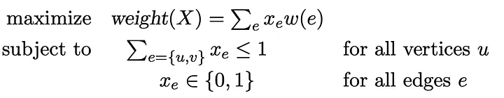
The objective function maximizes the weight of the edges in the matching, while the constraints limit us to one edge per vertex (no more than one assignment per driver and per rider).
In plain terms:
This mathematical formulation helps decide which driver gets paired with which rider to maximize overall benefit. We aim to select the matches that provide the highest total value, considering factors like proximity, pickup time, and cost. The first constraint ensures that no driver or rider is involved in more than one match — each person can only be matched once. Lastly, the variables can only be 0 or 1, meaning either the match happens or it doesn’t.
If we replace the 0–1 constraints on the selection variables with inequalities of the form 0 ≤ xₑ ≤1 we get the linear program relaxation of this ILP. We don’t need to include these inequalities explicitly, since the form of the standard linear program already constrains the xₑ to be non-negative and consequently, the other 2 constraints prevent them from being larger than 1. Dealing with the linear program (LP) relaxation instead of the original ILP is helpful because LPs are much faster and easier to solve. Furthermore, Edmonds shows that for bipartite graphs, the LP relaxation gives us integer solutions anyway, even though no explicit constraint on integrality is enforced. This enables the use of fast and efficient algorithms to solve the problem. Theoretically, the Hungarian algorithm solves the problem in polynomial time. In practice, commercial solvers are faster and can even handle some binary constraints (multiple routes, many-to-one matchings etc.)
Specificity of Lyft’s (or ridesharing in general) matching instances
Solving matching problems in the context of ridesharing presents significant challenges primarily due to the dynamic nature of the data, requiring the generation and processing of bipartite matching graphs at frequent intervals, such as every few seconds, on a rolling basis.
Each time we generate a graph, edge weights — reflecting factors like driver location, rider demand, and market conditions — must be recalculated to reflect the most current and accurate information. Because this data changes rapidly (drivers constantly on the move, demand levels fluctuating, traffic conditions), our system needs to update weights in real-time without excessive computational overhead. Achieving this requires efficient data handling and smart preprocessing to skip edges unlikely to be part of the optimal solution, balancing speed and accuracy.
Zoom image will be displayed
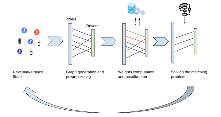
Figure 2: The cycle of generating and solving a matching problem.
When calculating matchings, we must carefully choose the time interval for batching nearby drivers and riders — a decision that delicately balances computational efficiency with service quality. Longer batches give a fuller picture of supply and demand, often producing better matches, lower wait times, and higher vehicle utilization, but they can delay ride assignments and risk cancellations. Shorter intervals speed up matches and keep riders and drivers engaged, but may lead to suboptimal pairings and higher computational demands. The challenge is finding the right frequency to maximize efficiency and customer satisfaction amid fluctuating demand, supply, and resource constraints.
Once we’ve set the batch size, we can compute the optimal matches for that snapshot using algorithms like the Hungarian method. However, optimizing each batch in isolation can be short-sighted, prioritizing immediate gains over long-term efficiency. A match that looks optimal now might increase wait times or reduce driver availability later. The figure below illustrates this: at time t=0, two drivers are available for one ride request, leading to the white car being dispatched. At t=1, a new request appears, but with only the black car left, resulting in a longer wait.
Zoom image will be displayed
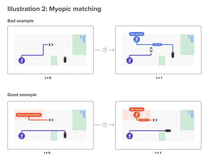
Figure 3: Example of how myopic decision making can lead to long term inefficiency.
To mitigate the sub-optimality arising from myopic matching between batches, several strategies can be adopted. For instance, we can use predictive analytics to forecast future demand and supply patterns, and augment the matching graph with the “projected future demand” from high density areas. In our example, this can reserve the white car for future batches, and result in a matching that minimizes the average waiting time. Other techniques can also include (1) incorporating long-term objectives in the weights of the matching graph, such as minimizing total wait time over a longer period or maximizing driver utilization rates, as well as (2) Dynamic Rebalancing, to continuously adjust the allocation of drivers based on real-time data, through incentives and bonuses.
To conclude, matching riders to drivers may seem straightforward, but doing it well — at scale, in real time, and under uncertainty — is a deeply complex optimization challenge. In this post, we introduced the core concepts behind how we model and solve matching problems at Lyft, highlighting both the mathematical structure and the practical constraints of real-world ridesharing systems.
In Part 2, we’ll explore how Machine Learning and Optimization work together to produce high-quality dispatch decisions, and discuss ongoing efforts to reduce the impact of uncertainty through forecasting, dynamic rebalancing, and smarter long-term decision-making.
Acknowledgments
We would like to thank Brian for his contributions in designing the graphs used in this post, as well as the editing team (Hongru, Jeana, Kelly, Miriam) for their thoughtful reviews and constructive feedback.
Lyft is hiring! If you’re passionate about solving this kind of optimization problem, visit https://www.lyft.com/careers to see our openings.