Inside GPT-OSS: OpenAI’s Latest LLM Architecture
[

Press enter or click to view image in full size
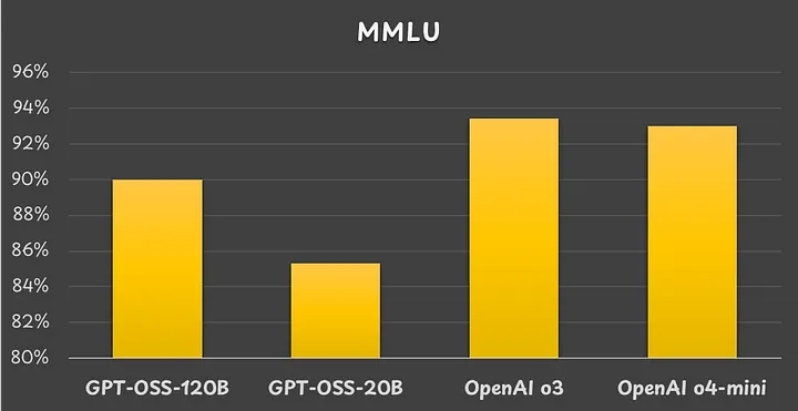
Massive Multitask Language Understanding (MMLU) benchmark results. Image by the author.
It has been several years since OpenAI shared information about how its LLMs work. Despite the word “open” in its name, OpenAI has not yet disclosed the inner workings of GPT-4 and GPT-5.
However, with the release of the open-weight GPT-OSS models, we finally have new information about OpenAI’s LLM design process.
To learn about the latest state-of-the-art LLM architecture, I recommend studying OpenAI’s GPT-OSS.
Overall LLM Model Architecture
To fully understand the LLM architecture, we must review OpenAI’s papers on GPT-1 [1], GPT-2 [2], GPT-3 [3], and GPT-OSS [4].
The overall LLM model architecture can be summarized as follows:
Press enter or click to view image in full size
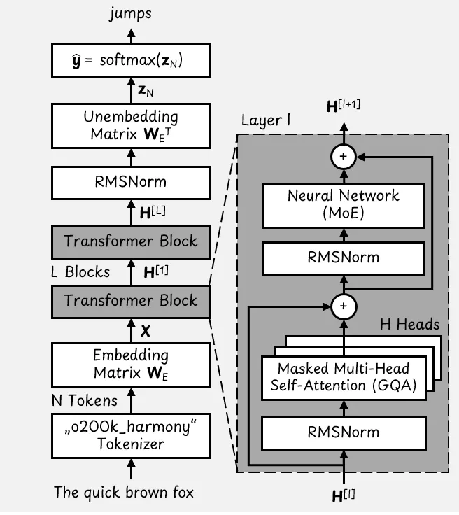
The basic GPT-OSS Transformer architecture. Image adapted from [5]
Based on this figure, we start at the bottom with an example input sentence, “The quick brown fox”. The goal of the LLM is to predict the next token, which could be “jumps”.
Tokenization
First, the tokenizer converts the input sentence into a list of N tokens. The o200k_harmony tokenizer is based on the byte pair encoding (BPE) algorithm [6] and has a vocabulary of 201,088 tokens.
This means that each token is a one-hot vector (with only one 1 and the rest zeros) of dimension |V| = 201,088. Thus, the input sentence becomes a matrix of shape [N x 201,088].
Token Embeddings
The embedding matrix transforms the list of tokens into a dense matrix of shape [N x D]. For GPT-OSS, the model dimension is D = 2,880. As a result, we end up with a matrix **X** of token embeddings with the shape [N x 2,880].
Transformer Blocks
A Transformer model consists of multiple layers of Transformer blocks:
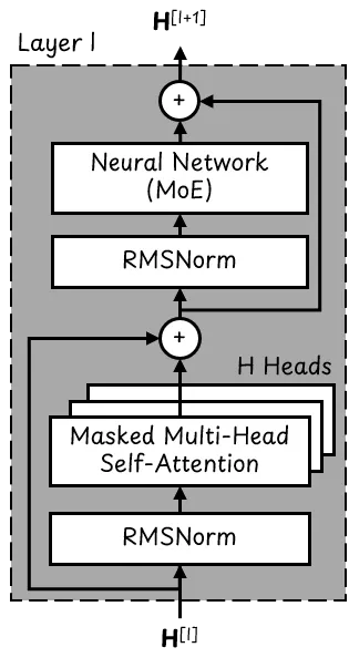
A single Transformer block. Image adapted from [5]
The token embeddings pass through these vertically stacked layers of Transformer blocks. GPT-OSS-20B has L = 24 layers, and GPT-OSS-120B has L = 36 layers.
Each Transformer block contains two layer normalization blocks that use RMSNorm [7] to ensure the values flowing through the Transformer remain within an appropriate range.
Each Transformer block also has H = 64 parallel attention heads and a Mixture of Experts (MoE) neural network. We will talk about this in more detail.
The input and output of each Transformer block is a matrix **H** of shape [N x 2,880].
Language Model Head
The language model head consists of the unembedding matrix and the final softmax layer. The unembedding matrix transforms the embedding vectors back into the token space. After unembedding, the resulting matrix has dimensions [N x 201,088].
The softmax layer converts each of the N token vectors (called logits) into probabilities. To predict the next token, we only need the last logit.
The final output is a vector of probabilities of size 201,088 (the size of the tokenizer’s vocabulary), which might tell us that the probability for the token “jumps” is 98%.
Mixture of Experts (MoE)
Recently, many large MoE models have emerged, including Qwen 3, Llama 4, DeepSeek V3, and Grok 3. So it’s no surprise that GPT-OSS is an MoE model as well.
A MoE layer replaces the standard neural network in the Transformer block. It consists of a router component and multiple neural networks, or “experts.”
The router, which is a small neural network, decides which expert should process each input token. Rather than selecting just one expert, the router selects multiple experts with different weights. For example, A = 0.7 x NN 2 + 0.3 x NN 4.
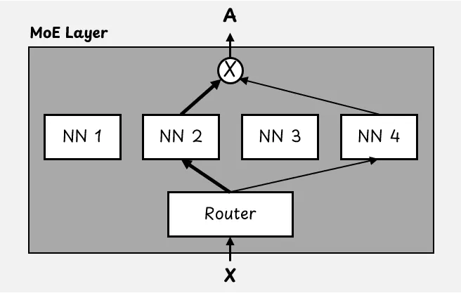
How a MoE layer works. In this example, the top 2 experts are used out of 4 experts. Image from [5]
In GPT-OSS, both models activate the top four experts. The total number of experts varies depending on the size of the model. For example, GPT-OSS-120B has 128 total experts, while GPT-OSS-20B has 32.
This is why MoE models have “active” and “total” parameters. During inference, the model only uses a few active neural networks in each MoE layer.
Quantization
Because MoE parameters account for over 90% of the total parameter count, they have been quantized to 4-bit floating-point numbers during the post-training process.
Specifically, OpenAI uses the MXFP4 format [8] for GPT-OSS, which uses 4 bits per parameter, and 32 parameters share the same scaling factor. The scaling factor is an 8-bit number, so that adds 8/32 = 0.25 bits per parameter. In total, that amounts to 4.25 bits per parameter, including the scaling factor.
Attention
GQA Attention
GPT-OSS uses Grouped-Query Attention (GQA) [9] instead of standard self-attention heads.
In standard multi-head attention, each attention head has a query matrix **W**_Q, a key matrix **W**_K, and a value matrix **W**_V.
Therefore, a model with H attention heads then requires 3H matrices to compute queries, keys, and values. This process becomes increasingly resource-intensive as the number of heads increases, especially in larger LLMs.
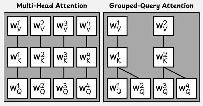
Standard multi-head attention vs. Grouped-Query Attention for H = 4 parallel attention heads. Image from [5]
For greater efficiency, multiple query heads in GQA share the same key and value heads.
In GPT-OSS, each attention layer has 64 query heads and 8 key-value heads.
Long Context Attention
Originally, positional encoding was added to the embedding vectors in the Transformer architecture. However, many modern LLMs, including GPT-OSS, have used Rotary Positional Encodings (RoPE) instead.
RoPE [10] rotates the query and key vectors within the attention mechanism to incorporate positional information about the tokens. A token’s position within an input sequence can be described by an integer k, where k = 0 for the first token, k = 1 for the second token, and so on.
RoPE rotates a given vector counterclockwise by an angle that depends on the token’s position.
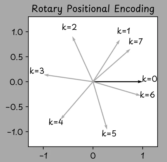
The two-dimensional embedding vector is rotated counterclockwise by an angle that depends on the token’s position k in the input sequence. Image from [5]
GPT-OSS uses and extends RoPE for context lengths of up to 131,072 tokens.
GPT-OSS also uses a technique called banded window attention for long context input.
In standard masked self-attention, each token can “look” at itself and at all preceding tokens. With N tokens in an input sequence, an N x N attention matrix is created. The longer the context length of the LLM, the more problematic this becomes.
In a sparse attention mechanism [11], there is a limit to how far back a token can “look”. In GPT-OSS, this limit or attention window is 128 tokens long.
Press enter or click to view image in full size
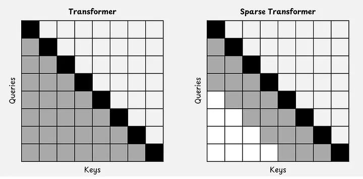
Normal attention vs. sparse attention mechanism [11]. A query can only look at keys before it (black and gray). Image by the author.
GPT-OSS alternates between full attention, which considers the entire global context, and “banded window” attention, which only considers a small local part of the text.
Conclusion
After GPT-3, we finally got a new update from OpenAI. This update gives us a peek at their current LLM architecture.
There is nothing surprising or new in GPT-OSS. As it turns out, it is actually very similar to other recently released LLMs, for example, Qwen 3 [12]. In fact, the architecture of GPT-OSS-20B is nearly identical to that of Qwen3–30B-A3B.
It’s reasonable to assume that GPT-4 and GPT-5 have similar architectures, just scaled up significantly. Either that or OpenAI has some hidden tricks that they did not reveal with GPT-OSS. However, I don’t think that is very likely.
The model’s performance is impacted by more than just the LLM’s architecture; the training data and the training process also play a role. Perhaps this is where OpenAI’s models truly excel.