Building an Image Hashing Search Engine with VP-Trees and OpenCV
In this tutorial, you will learn how to build a scalable image hashing search engine using OpenCV, Python, and VP-Trees.
Image hashing algorithms are used to:
- Uniquely quantify the contents of an image using only a single integer.
- Find duplicate or near-duplicate images in a dataset of images based on their computed hashes.
Back in 2017, I wrote a tutorial on image hashing with OpenCV and Python (which is required reading for this tutorial). That guide showed you how to find identical/duplicate images in a given dataset.
However, there was a scalability problem with that original tutorial — namely that it did not scale!
To find near-duplicate images, our original image hashing method would require us to perform a linear search, comparing the query hash to each individual image hash in our dataset.
In a practical, real-world application that’s far too slow — we need to find a way to reduce that search to sub-linear time complexity.
But how can we reduce search time so dramatically?
The answer is a specialized data structure called a VP-Tree.
Using a VP-Tree we can reduce our search complexity from O(n) to O(log n), enabling us to obtain our sub-linear goal!
In the remainder of this tutorial you will learn how to:
- Build an image hashing search engine to find both identical and near-identical images in a dataset.
- Utilize a specialized data structure, called a VP-Tree, that can be used used to scale image hashing search engines to millions of images.
To learn how to build your first image hashing search engine with OpenCV, just keep reading!
In the first part of this tutorial, I’ll review what exactly an image search engine is for newcomers to PyImageSearch.
Then, we’ll discuss the concept of image hashing and perceptual hashing, including how they can be used to build an image search engine.
We’ll also take a look at problems associated with image hashing search engines, including algorithmic complexity.
Note: If you haven’t read my tutorial on Image Hashing with OpenCV and Python, make sure you do so now. That guide is required reading before you continue here.
From there, we’ll briefly review Vantage-point Trees (VP-Trees) which can be used to dramatically improve the efficiency and performance of image hashing search engines.
Armed with our knowledge we’ll implement our own custom image hashing search engine using VP-Trees and then examine the results.
What is an image search engine?
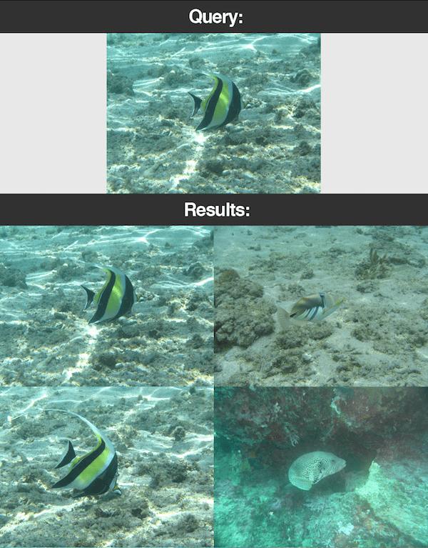
Figure 1: An example of an image search engine. A query image is presented and the search engine finds similar images in a dataset.
In this section, we’ll review the concept of an image search engine and direct you to some additional resources.
PyImageSearch has roots in image search engines — that was my main interest when I started the blog back in 2014. This tutorial is a fun one for me to share as I have a soft spot for image search engines as a computer vision topic.
Image search engines are a lot like textual search engines, only instead of using text as a query, we instead use an image.
When you use a text search engines, such as Google, Bing, or DuckDuckGo, etc., you enter your search query — a word or phrase. Indexed websites of interest are returned to you as results, and ideally, you’ll find what you are looking for.
Similarly, for an image search engine, you present a query image (not a textual word/phrase). The image search engine then returns similar image results based solely on the contents of the image.
Of course, there is a lot that goes on under the hood in any type of search engine — just keep this key concept of query/results in mind going forward as we build an image search engine today.
To learn more about image search engines, I suggest you refer to the following resources:
Read those guides to obtain a basic understanding of what an image search engine is, then come back to this post to learn about image hash search engines.
What is image hashing/perceptual hashing?
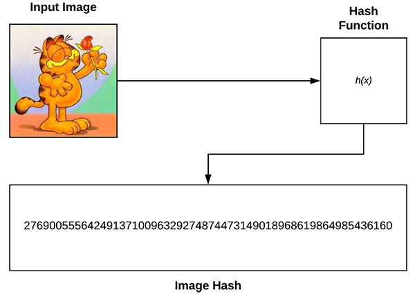
Figure 2: An example of an image hashing function. Top-left: An input image. Top-right: An image hashing function. Bottom: The resulting hash value. We will build a basic image hashing search engine with VP-Trees and OpenCV in this tutorial.
Image hashing, also called perceptual hashing, is the process of:
- Examining the contents of an image.
- Constructing a hash value (i.e., an integer) that uniquely quantifies an input image based on the contents of the image alone.
One of the benefits of using image hashing is that the resulting storage used to quantify the image is super small.
For example, let’s suppose we have an 800x600px image with 3 channels. If we were to store that entire image in memory using an 8-bit unsigned integer data type, the image would require 1.44MB of RAM.
Of course, we would rarely, if ever, store the raw image pixels when quantifying an image.
Instead, we would use algorithms such as keypoint detectors and local invariant descriptors (i.e., SIFT, SURF, etc.).
Applying these methods can typically lead to 100s to 1000s of features per image.
If we assume a modest 500 keypoints detected, each resulting in a feature vector of 128-d with a 32-bit floating point data type, we would require a total of 0.256MB to store the quantification of each individual image in our dataset.
Image hashing, on the other hand, allows us to quantify an image using only a 32-bit integer, requiring only 4 bytes of memory!

Figure 3: An image hash requires far less disk space in comparison to the original image bitmap size or image features (SIFT, etc.). We will use image hashes as a basis for an image search engine with VP-Trees and OpenCV.
Furthermore, image hashes should also be comparable.
Let’s suppose we compute image hashes for three input images, two of which near-identical images:
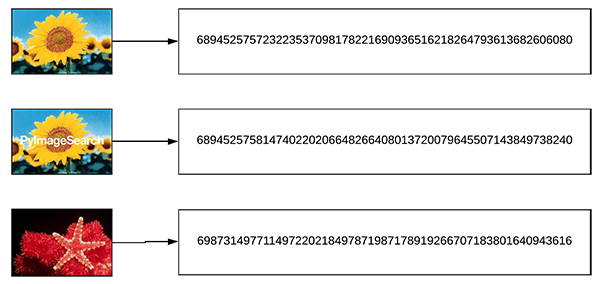
Figure 4: Three images with different hashes. The Hamming Distance between the top two hashes is closer than the Hamming distance to the third image. We will use a VP-Tree data structure to make an image hashing search engine.
To compare our image hashes we will use the Hamming distance. The Hamming distance, in this context, is used to compare the number of different bits between two integers.
In practice, this means that we count the number of 1s when taking the XOR between two integers.
Therefore, going back to our three input images above, the Hamming distance between our two similar images should be smaller (indicating more similarity) than the Hamming distance between the third less similar image:

Figure 5: The Hamming Distance between image hashes is shown. Take note that the Hamming Distance between the first two images is smaller than that of the first and third (or 2nd and 3rd). The Hamming Distance between image hashes will play a role in our image search engine using VP-Trees and OpenCV.
Again, note how the Hamming distance between the two images is smaller than the distances between the third image:
- The smaller the Hamming distance is between two hashes, the more similar the images are.
- And conversely, the larger the Hamming distance is between two hashes, the less similar the images are.
Also note how the distance between identical images (i.e., along the diagonal of Figure 5) are all zero — the Hamming distance between two hashes will be zero if the two input images are identical, otherwise the distance will be > 0, with larger values indicating less similarity.
There are a number of image hashing algorithms, but one of the most popular ones is called the difference hash, which includes four steps:
- Step #1: Convert the input image to grayscale.
- Step #2: Resize the image to fixed dimensions, N + 1 x N, ignoring aspect ratio. Typically we set N=8 or N=16. We use N + 1 for the number of rows so that we can compute the difference (hence “difference hash”) between adjacent pixels in the image.
- Step #3: Compute the difference. If we set N=8 then we have 9 pixels per row and 8 pixels per column. We can then compute the difference between adjacent column pixels, yielding 8 differences. 8 rows of 8 differences (i.e., 8×8) results in 64 values.
- Step #4: Finally, we can build the hash. In practice all we actually need to perform is a “greater than” operation comparing the columns, yielding binary values. These 64 binary values are compacted into an integer, forming our final hash.
Typically, image hashing algorithms are used to find near-duplicate images in a large dataset.
I’ve covered image hashing in detail inside this tutorial so if the concept is new to you, I would suggest reading that guide before continuing here.
What is an image hashing search engine?
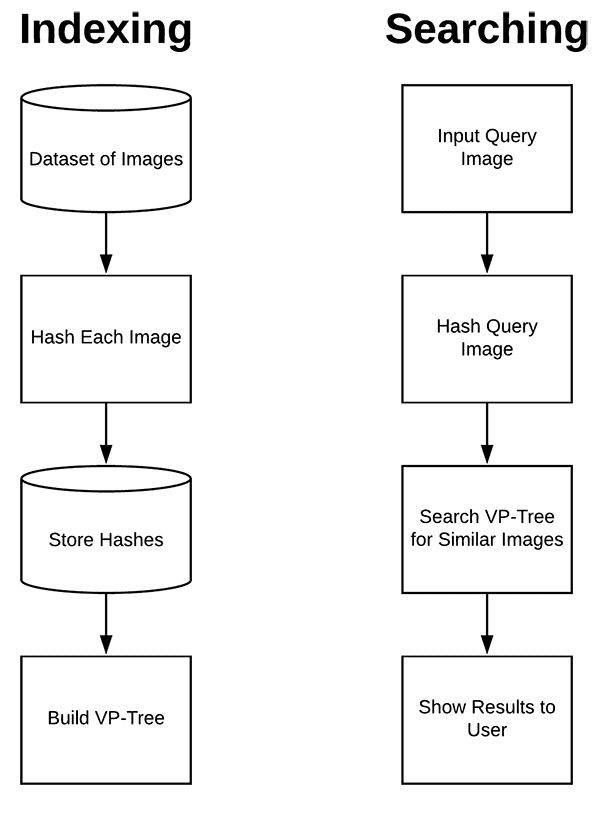
Figure 6: Image search engines consist of images, an indexer, and a searcher. We’ll index all of our images by computing and storing their hashes. We’ll build a VP-Tree of the hashes. The searcher will compute the hash of the query image and search the VP tree for similar images and return the closest matches. Using Python, OpenCV, and vptree, we can implement our image hashing search engine.
An image hashing search engine consists of two components:
- Indexing: Taking an input dataset of images, computing the hashes, and storing them in a data structure to facilitate fast, efficient search.
- Searching/Querying: Accepting an input query image from the user, computing the hash, and finding all near-identical images in our indexed dataset.
A great example of an image hashing search engine is TinEye, which is actually a reverse image search engine.
A reverse image search engine:
- Accepts an input image.
- Finds all near-duplicates of that image on the web, telling you the website/URL of where the near duplicate can be found.
Using this tutorial you will learn how to build your own TinEye!
What makes scaling image hashing search engines problematic?
One of the biggest issues with building an image hashing search engine is scalability — the more images you have, the longer it can take to perform the search.
For example, let’s suppose we have the following scenario:
- We have a dataset of 1,000,000 images.
- We have already computed image hashes for each of these 1,000,000 images.
- A user comes along, presents us with an image, and then asks us to find all near-identical images in that dataset.
How might you go about performing that search?
Would you loop over all 1,000,000 image hashes, one by one, and compare them to the hash of the query image?
Unfortunately, that’s not going to work. Even if you assume that each Hamming distance comparison takes 0.00001 seconds, with a total 1,000,000 images, it would take you 10 seconds to complete the search — far too slow for any type of search engine.
Instead, to build an image hashing search engine that scales, you need to utilize specialized data structures.
What are VP-Trees and how can they help scale image hashing search engines?

Figure 7: We’ll use VP-Trees for our image hash search engine using Python and OpenCV. VP-Trees are based on a recursive algorithm that computes vantage points and medians until we reach child nodes containing an individual image hash. Child nodes that are closer together (i.e. smaller Hamming Distances in our case) are assumed to be more similar to each other. (image source)
In order to scale our image hashing search engine, we need to use a specialized data structure that:
- Reduces our search from linear complexity,
O(n)… - …down to sub-linear complexity, ideally
O(log n).
To accomplish that task we can use Vantage-point Trees (VP-Trees). VP-Trees are a metric tree that operates in a metric space by selecting a given position in space (i.e., the “vantage point”) and then partitioning the data points into two sets:
- Points that are near the vantage point
- Points that are far from the vantage point
We then recursively apply this process, partitioning the points into smaller and smaller sets, thus creating a tree where neighbors in the tree have smaller distances.
To visualize the process of constructing a VP-Tree, consider the following figure:
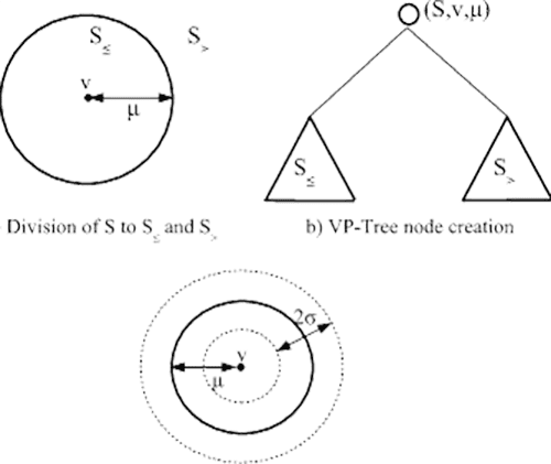
Figure 8: A visual depiction of the process of building a VP-Tree (vantage point tree). We will use the vptree Python implementation by Richard Sjogren. (image source)
First, we select a point in space (denoted as the v in the center of the circle) — we call this point the vantage point. The vantage point is the point furthest from the parent vantage point in the tree.
We then compute the median, μ, for all points, X.
Once we have μ, we then divide X into two sets, S1 and S2:
- All points with distance <= μ belong to S1.
- All points with distance > μ belong to S2.
We then recursively apply this process, building a tree as we go, until we are left with a child node.
A child node contains only a single data point (in this case, one individual hash). Child nodes that are closer together in the tree thus have:
- Smaller distances between them.
- And therefore assumed to be more similar to each other than the rest of the data points in the tree.
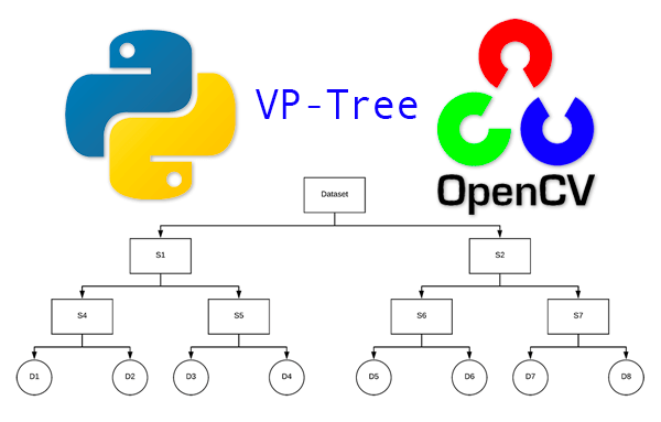
After recursively applying the VP-Tree construction method, we end up with a data structure, that, as the name suggests, is a tree:
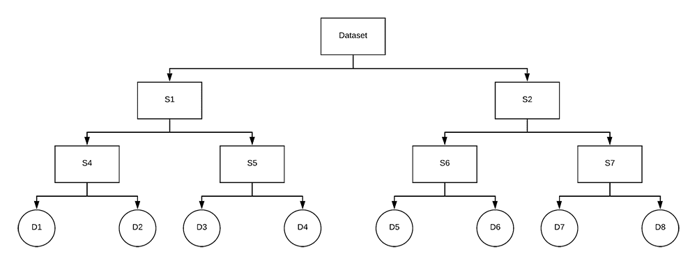
Figure 9: An example VP-Tree is depicted. We will use Python to build VP-Trees for use in an image hash search engine.
Notice how we recursively split subsets of our dataset into smaller and smaller subsets, until we eventually reach the child nodes.
VP-Trees take O(n log n) to build, but once we’ve constructed it, a search takes only O(log n), thus reducing our search time to sub-linear complexity!
Later in this tutorial, you’ll learn to utilize VP-Trees with Python to build and scale our image hashing search engine.
Note: This section is meant to be a gentle introduction to VP-Trees. If you are interested in learning more about them, I would recommend (1) consulting a data structures textbook, (2) following this guide from Steve Hanov’s blog, or (3) reading this writeup from Ivan Chen.
The CALTECH-101 dataset
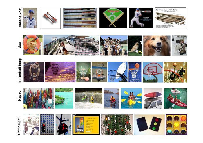
Figure 10: The CALTECH-101 dataset consists of 101 object categories. Our image hash search engine using VP-Trees, Python, and OpenCV will use the CALTECH-101 dataset for our practical example.
The dataset we’ll be working today is the CALTECH-101 dataset which consists of 9,144 total images across 101 categories (with 40 to 800 images per category).
The dataset is large enough to be interesting to explore from an introductory to image hashing perspective but still small enough that you can run the example Python scripts in this guide without having to wait hours and hours for your system to finish chewing on the images.
You can download the CALTECH 101 dataset from their official webpage or you can use the following wget command:
$ wget http://www.vision.caltech.edu/Image_Datasets/Caltech101/101_ObjectCategories.tar.gz $ tar xvzf 101_ObjectCategories.tar.gz
Project structure
Let’s inspect our project structure:
$ tree --dirsfirst . ├── pyimagesearch │ ├── __init__.py │ └── hashing.py ├── 101_ObjectCategories [9,144 images] ├── queries │ ├── accordion.jpg │ ├── accordion_modified1.jpg │ ├── accordion_modified2.jpg │ ├── buddha.jpg │ └── dalmation.jpg ├── index_images.py └── search.py
The pyimagesearch module contains hashing.py which includes three hashing functions. We will review the functions in the “Implementing our hashing utilities” section below.
Our dataset is in the 101_ObjectCategories/ folder (CALTECH-101) contains 101 sub-directories with our images. Be sure to read the previous section to learn how to download the dataset.
There are five query images in the queries/ directory. We will search for images with similar hashes to these images. The accordion_modified1.jpg and accordion_modiied2.jpg images will present unique challenges to our VP-Trees image hashing search engine.
The core of today’s project lies in two Python scripts: index_images.py and search.py :
- Our indexer will calculate hashes for all 9,144 images and organize the hashes in a VP-Tree. This index will reside in two
.picklefiles: (1) a dictionary of all computed hashes, and (2) the VP-Tree. - The searcher will calculate the hash for a query image and search the VP-Tree for the closest images via Hamming Distance. The results will be returned to the user.
If that sounds like a lot, don’t worry! This tutorial will break everything down step-by-step.
Configuring your development environment
For this blog post, your development environment needs the following packages installed:
Luckily for us, everything is pip-installable. My recommendation for you is to follow the first OpenCV link to pip-install OpenCV in a virtual environment on your system. From there you’ll just pip-install everything else in the same environment.
It will look something like this:
# setup pip, virtualenv, and virtualenvwrapper (using the "pip install OpenCV" instructions) $ workon <env_name> $ pip install numpy $ pip install opencv-contrib-python $ pip install imutils $ pip install vptree
Replace <env_name> with the name of your virtual environment. The workon command will only be available once you set up virtualenv and virtualenvwrapper following these instructions.
Implementing our image hashing utilities
Before we can build our image hashing search engine, we first need to implement a few helper utilities.
Open up the hashing.py file in the project structure and insert the following code:
# import the necessary packages import numpy as np import cv2
def dhash(image, hashSize=8):
convert the image to grayscale
gray = cv2.cvtColor(image, cv2.COLOR_BGR2GRAY)
resize the grayscale image, adding a single column (width) so we
can compute the horizontal gradient
resized = cv2.resize(gray, (hashSize + 1, hashSize))
compute the (relative) horizontal gradient between adjacent
column pixels
diff = resized[:, 1:] > resized[:, :-1]
convert the difference image to a hash
return sum([2 ** i for (i, v) in enumerate(diff.flatten()) if v])
We begin by importing OpenCV and NumPy (Lines 2 and 3).
The first function we’ll look at, dhash, is used to compute the difference hash for a given input image. Recall from above that our dhash requires four steps: (1) convert to grayscale, (2) resize, (3) compute the difference, and (4) build the hash. Let’s break it down a little further:
- Line 7 converts the image to grayscale.
- Line 11 resizes the image to N + 1 rows by N columns, ignoring the aspect ratio. This ensures that the resulting image hash will match similar photos regardless of their initial spatial dimensions.
- Line 15 computes the horizontal gradient difference between adjacent column pixels. Assuming
hashSize=8, will be 8 rows of 8 differences (there are 9 rows allowing for 8 comparisons). We will thus have a 64-bit hash as 8×8=64. - Line 18 converts the difference image to a hash.
For more details, refer to this blog post.
Next, let’s look at convert_hash function:
def convert_hash(h):
convert the hash to NumPy's 64-bit float and then back to
Python's built in int
return int(np.array(h, dtype="float64"))
When I first wrote the code for this tutorial, I found that the VP-Tree implementation we’re using internally converts points to a NumPy 64-bit float. That would be okay; however, hashes need to be integers and if we convert them to 64-bit floats, they become an unhashable data type. To overcome the limitation of the VP-Tree implementation, I came up with the convert_hash hack:
- We accept an input hash,
h. - That hash is then converted to a NumPy 64-bit float.
- And that NumPy float is then converted back to Python’s built-in integer data type.
This hack ensures that hashes are represented consistently throughout the hashing, indexing, and searching process.
We then have one final helper method, hamming, which is used to compute the Hamming distance between two integers:
def hamming(a, b):
compute and return the Hamming distance between the integers
return bin(int(a) ^ int(b)).count("1")
The Hamming distance is simply a count of the number of 1s when taking the XOR (^) between two integers (Line 27).
Implementing our image hash indexer
Before we can perform a search, we first need to:
- Loop over our input dataset of images.
- Compute difference hash for each image.
- Build a VP-Tree using the hashes.
Let’s start that process now.
Open up the index_images.py file and insert the following code:
# import the necessary packages from pyimagesearch.hashing import convert_hash from pyimagesearch.hashing import hamming from pyimagesearch.hashing import dhash from imutils import paths import argparse import pickle import vptree import cv2
construct the argument parser and parse the arguments
ap = argparse.ArgumentParser() ap.add_argument("-i", "--images", required=True, type=str, help="path to input directory of images") ap.add_argument("-t", "--tree", required=True, type=str, help="path to output VP-Tree") ap.add_argument("-a", "--hashes", required=True, type=str, help="path to output hashes dictionary") args = vars(ap.parse_args())
Lines 2-9 import the packages, functions, and modules necessary for this script. In particular Lines 2-4 import our three hashing related functions: convert_hash , hamming , and dhash . Line 8 imports the vptree implementation that we will be using.
Next, Lines 12-19 parse our command line arguments:
--images: The path to our images which we will be indexing.--tree: The path to the output VP-tree.picklefile which will be serialized to disk.--hashes: The path to the output hashes dictionary which will be stored in.pickleformat.
Now let’s compute hashes for all images:
# grab the paths to the input images and initialize the dictionary
of hashes
imagePaths = list(paths.list_images(args["images"])) hashes = {}
loop over the image paths
for (i, imagePath) in enumerate(imagePaths):
load the input image
print("[INFO] processing image {}/{}".format(i + 1, len(imagePaths))) image = cv2.imread(imagePath)
compute the hash for the image and convert it
h = dhash(image) h = convert_hash(h)
update the hashes dictionary
l = hashes.get(h, []) l.append(imagePath) hashes[h] = l
Lines 23 and 24 grab image paths and initialize our hashes dictionary.
Line 27 then begins a loop over all the imagePaths . Inside the loop, we:
- Load the
image(Line 31). - Compute and convert the hash,
h(Lines 34 and 35). - Grab a list of all image paths,
l, with the same hash (Line 38). - Add this
imagePathto the list,l(Line 39). - Update our dictionary with the hash as the key and our list of image paths with the same corresponding hash as the value (Line 40).
From here, we build our VP-Tree:
# build the VP-Tree print("[INFO] building VP-Tree...") points = list(hashes.keys()) tree = vptree.VPTree(points, hamming)
To construct the VP-Tree, Lines 44 and 45 pass in (1) a list of data points (i.e., the hash integer values themselves), and (2) our distance function (the Hamming distance method) to the VPTree constructor.
Internally, the VP-Tree computes the Hamming distances between all input points and then constructs the VP-Tree such that data points with smaller distances (i.e., more similar images) lie closer together in the tree space. Be sure to refer the “What are VP-Trees and how can they help scale image hashing search engines?” section and Figures 7, 8, and 9.
With our hashes dictionary populated and VP-Tree constructed, we’ll now serialize them both to disk as .pickle files:
# serialize the VP-Tree to disk print("[INFO] serializing VP-Tree...") f = open(args["tree"], "wb") f.write(pickle.dumps(tree)) f.close()
serialize the hashes to dictionary
print("[INFO] serializing hashes...") f = open(args["hashes"], "wb") f.write(pickle.dumps(hashes)) f.close()
Extracting image hashes and building the VP-Tree
Now that we’ve implemented our indexing script, let’s put it to work. Make sure you’ve:
- Downloaded the CALTECH-101 dataset using the instructions above.
- Used the “Downloads” section of this tutorial to download the source code and example query images.
- Extracted the .zip of the source code and changed directory to the project.
From there, open up a terminal and issue the following command:
$ time python index_images.py --images 101_ObjectCategories \ --tree vptree.pickle --hashes hashes.pickle [INFO] processing image 1/9144 [INFO] processing image 2/9144 [INFO] processing image 3/9144 [INFO] processing image 4/9144 [INFO] processing image 5/9144 ... [INFO] processing image 9140/9144 [INFO] processing image 9141/9144 [INFO] processing image 9142/9144 [INFO] processing image 9143/9144 [INFO] processing image 9144/9144 [INFO] building VP-Tree... [INFO] serializing VP-Tree... [INFO] serializing hashes...
real0m10.947s user0m9.096s sys0m1.386s
As our output indicates, we were able to hash all 9,144 images in just over 10 seconds.
Checking project directory after running the script we’ll find two .pickle files:
$ ls -l *.pickle -rw-r--r-- 1 adrianrosebrock 796620 Aug 22 07:53 hashes.pickle -rw-r--r-- 1 adrianrosebrock 707926 Aug 22 07:53 vptree.pickle
The hashes.pickle (796.62KB) file contains our computed hashes, mapping the hash integer value to file paths with the same hash. The vptree.pickle (707.926KB) is our constructed VP-Tree.
We’ll be using this VP-Tree to perform queries and searches in the following section.
Implementing our image hash searching script
The second component of an image hashing search engine is the search script. The search script will:
- Accept an input query image.
- Compute the hash for the query image.
- Search the VP-Tree using the query hash to find all duplicate/near-duplicate images.
Let’s implement our image hash searcher now — open up the search.py file and insert the following code:
# import the necessary packages from pyimagesearch.hashing import convert_hash from pyimagesearch.hashing import dhash import argparse import pickle import time import cv2
construct the argument parser and parse the arguments
ap = argparse.ArgumentParser() ap.add_argument("-t", "--tree", required=True, type=str, help="path to pre-constructed VP-Tree") ap.add_argument("-a", "--hashes", required=True, type=str, help="path to hashes dictionary") ap.add_argument("-q", "--query", required=True, type=str, help="path to input query image") ap.add_argument("-d", "--distance", type=int, default=10, help="maximum hamming distance") args = vars(ap.parse_args())
Lines 2-9 import the necessary components for our searching script. Notice that we need the dhash and convert_hash functions once again as we’ll have to compute the hash for our --query image.
Lines 10-19 parse our command line arguments (the first three are required):
--tree: The path to our pre-constructed VP-Tree on disk.--hashes: The path to our pre-computed hashes dictionary on disk.--query: Our query image’s path.--distance: The maximum hamming distance between hashes is set with adefaultof10. You may override it if you so choose.
It’s important to note that the larger the --distance is, the more hashes the VP-Tree will compare, and thus the searcher will be slower. Try to keep your --distance as small as possible without compromising the quality of your results.
Next, we’ll (1) load our VP-Tree + hashes dictionary, and (2) compute the hash for our --query image:
# load the VP-Tree and hashes dictionary print("[INFO] loading VP-Tree and hashes...") tree = pickle.loads(open(args["tree"], "rb").read()) hashes = pickle.loads(open(args["hashes"], "rb").read())
load the input query image
image = cv2.imread(args["query"]) cv2.imshow("Query", image)
compute the hash for the query image, then convert it
queryHash = dhash(image) queryHash = convert_hash(queryHash)
Lines 23 and 24 load the pre-computed index including the VP-Tree and hashes dictionary.
From there, we load and display the --query image (Lines 27 and 28).
We then take the query image and compute the queryHash (Lines 31 and 32).
At this point, it is time to perform a search using our VP-Tree:
# perform the search print("[INFO] performing search...") start = time.time() results = tree.get_all_in_range(queryHash, args["distance"]) results = sorted(results) end = time.time() print("[INFO] search took {} seconds".format(end - start))
Lines 37 and 38 perform a search by querying the VP-Tree for hashes with the smallest Hamming distance relative to the queryHash . The results are sorted so that “more similar” hashes are at the front of the results list.
Both of these lines are sandwiched with timestamps for benchmarking purposes, the results of which are printed via Line 40.
Finally, we will loop over results and display each of them:
# loop over the results for (d, h) in results:
grab all image paths in our dataset with the same hash
resultPaths = hashes.get(h, []) print("[INFO] {} total image(s) with d: {}, h: {}".format( len(resultPaths), d, h))
loop over the result paths
for resultPath in resultPaths:
load the result image and display it to our screen
result = cv2.imread(resultPath) cv2.imshow("Result", result) cv2.waitKey(0)
Line 43 begins a loop over the results :
- The
resultPathsfor the current hash,h, are grabbed from the hashes dictionary (Line 45). - Each
resultimage is displayed as a key is pressed on the keyboard (Lines 50-54).
Image hashing search engine results
We are now ready to test our image search engine!
But before we do that, make sure you have:
- Downloaded the CALTECH-101 dataset using the instructions above.
- Used the “Downloads” section of this tutorial to download the source code and example query images.
- Extracted the .zip of the source code and changed directory to the project.
- Ran the
index_images.pyfile to generate thehashes.pickleandvptree.picklefiles.
After all the above steps are complete, open up a terminal and execute the following command:
python search.py --tree vptree.pickle --hashes hashes.pickle \ --query queries/buddha.jpg [INFO] loading VP-Tree and hashes... [INFO] performing search... [INFO] search took 0.015203237533569336 seconds [INFO] 1 total image(s) with d: 0, h: 8.162938100012111e+18
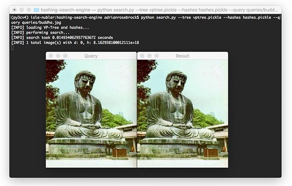
Figure 11: Our Python + OpenCV image hashing search engine found a match in the VP-Tree in just 0.015 seconds!
On the left, you can see our input query image of our Buddha. On the right, you can see that we have found the duplicate image in our indexed dataset.
The search itself took only 0.015 seconds.
Additionally, note that the distance between the input query image and the hashed image in the dataset is zero, indicating that the two images are identical.
Let’s try again, this time with an image of a Dalmatian:
$ python search.py --tree vptree.pickle --hashes hashes.pickle \ --query queries/dalmation.jpg [INFO] loading VP-Tree and hashes... [INFO] performing search... [INFO] search took 0.014827728271484375 seconds [INFO] 1 total image(s) with d: 0, h: 6.445556196029652e+18
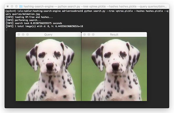
Figure 12: With a Hamming Distance of 0, the Dalmation query image yielded an identical image in our dataset. We built an OpenCV + Python image hash search engine with VP-Trees successfully.
Again, we see that our image hashing search engine has found the identical Dalmatian in our indexed dataset (we know the images are identical due to the Hamming distance of zero).
The next example is of an accordion:
$ python search.py --tree vptree.pickle --hashes hashes.pickle \ --query queries/accordion.jpg [INFO] loading VP-Tree and hashes... [INFO] performing search... [INFO] search took 0.014187097549438477 seconds [INFO] 1 total image(s) with d: 0, h: 3.380309217342405e+18
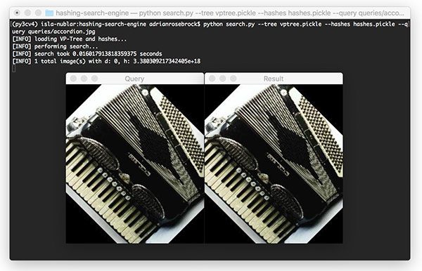
Figure 13: An example of providing a query image and finding the best resulting image with an image hash search engine created with Python and OpenCV.
We once again find our identical matched image in the indexed dataset.
We know our image hashing search engine is working great for identical images…
…but what about images that are slightly modified?
Will our hashing search engine still perform well?
Let’s give it a try:
$ python search.py --tree vptree.pickle --hashes hashes.pickle \ --query queries/accordion_modified1.jpg [INFO] loading VP-Tree and hashes... [INFO] performing search... [INFO] search took 0.014217138290405273 seconds [INFO] 1 total image(s) with d: 4, h: 3.380309217342405e+18

Figure 14: Our image hash search engine was able to find the matching image despite a modification (red square) to the query image.
Here I’ve added a small red square in the bottom left corner of the accordion query image. This addition will change the difference hash value!
However, if you take a look at the output result, you’ll see that we were still able to detect the near-duplicate image.
We were able to find the near-duplicate image by comparing the Hamming distance between the hashes. The difference in hash values is 4, indicating that 4 bits differ between the two hashes.
Next, let’s try a second query, this one much more modified than the first:
$ python search.py --tree vptree.pickle --hashes hashes.pickle \ --query queries/accordion_modified2.jpg [INFO] loading VP-Tree and hashes... [INFO] performing search... [INFO] search took 0.013727903366088867 seconds [INFO] 1 total image(s) with d: 9, h: 3.380309217342405e+18
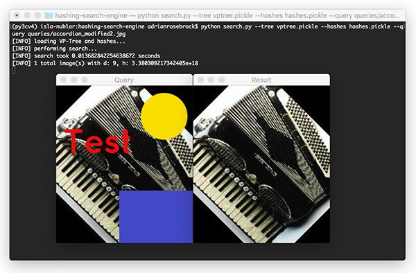
Figure 15: On the left is the query image for our image hash search engine with VP-Trees. It has been modified with yellow and purple shapes as well as red text. The image hash search engine returns the correct resulting image (right) from an index of 9,144 in just 0.0137 seconds, proving the robustness of our search engine system.
Despite dramatically altering the query by adding in a large blue rectangle, a yellow circle, and text, we’re still able to find the near-duplicate image in our dataset in under 0.014 seconds!
Whenever you need to find duplicate or near-duplicate images in a dataset, definitely consider using image hashing and image searching algorithms — when used correctly, they can be extremely powerful!

Course information: 25 total classes • 37h 19m video • Last updated: 7/2021
★★★★★ 4.84 (128 Ratings) • 10,597 Students Enrolled
I strongly believe that if you had the right teacher you could master computer vision and deep learning.
Do you think learning computer vision and deep learning has to be time-consuming, overwhelming, and complicated? Or has to involve complex mathematics and equations? Or requires a degree in computer science?
That’s not the case.
All you need to master computer vision and deep learning is for someone to explain things to you in simple, intuitive terms. And that’s exactly what I do. My mission is to change education and how complex Artificial Intelligence topics are taught.
If you're serious about learning computer vision, your next stop should be PyImageSearch University, the most comprehensive computer vision, deep learning, and OpenCV course online today. Here you’ll learn how to successfully and confidently apply computer vision to your work, research, and projects. Join me in computer vision mastery.
Inside PyImageSearch University you'll find:
- ✓ 25 courses on essential computer vision, deep learning, and OpenCV topics
- ✓ 25 Certificates of Completion
- ✓ 37h 19m on-demand video
- ✓ Brand new courses released every month, ensuring you can keep up with state-of-the-art techniques
- ✓ Pre-configured Jupyter Notebooks in Google Colab
- ✓ Run all code examples in your web browser — works on Windows, macOS, and Linux (no dev environment configuration required!)
- ✓ Access to centralized code repos for all 400+ tutorials on PyImageSearch
- ✓ Easy one-click downloads for code, datasets, pre-trained models, etc.
- ✓ Access on mobile, laptop, desktop, etc.
Click here to join PyImageSearch University
Summary
In this tutorial, you learned how to build a basic image hashing search engine using OpenCV and Python.
To build an image hashing search engine that scaled we needed to utilize VP- Trees, a specialized metric tree data structure that recursively partitions a dataset of points such that nodes of the tree that are closer together are more similar than nodes that are farther away.
By using VP-Trees we were able to build an image hashing search engine capable of finding duplicate and near-duplicate images in a dataset in under 0.01 seconds.
Furthermore, we demonstrated that our combination of hashing algorithm and VP-Tree search was capable of finding matches in our dataset, even if our query image was modified, damaged, or altered!
If you are ever building a computer vision application that requires quickly finding duplicate or near-duplicate images in a large dataset, definitely give this method a try.
To download the source code to this post, and be notified when future posts are published here on PyImageSearch, just enter your email address in the form below!

Enter your email address below to get a .zip of the code and a FREE 17-page Resource Guide on Computer Vision, OpenCV, and Deep Learning. Inside you'll find my hand-picked tutorials, books, courses, and libraries to help you master CV and DL!