How-To: OpenCV and Python K-Means Color Clustering

Take a second to look at the Jurassic Park movie poster above.
What are the dominant colors? (i.e. the colors that are represented most in the image)
Well, we see that the background is largely black. There is some red around the T-Rex. And there is some yellow surrounding the actual logo.
It’s pretty simple for the human mind to pick out these colors.
But what if we wanted to create an algorithm to automatically pull out these colors?
You might think that a color histogram is your best bet…
But there’s actually a more interesting algorithm we can apply — k-means clustering.
In this blog post I’ll show you how to use OpenCV, Python, and the k-means clustering algorithm to find the most dominant colors in an image.
OpenCV and Python versions:
This example will run on Python 2.7/Python 3.4+ and OpenCV 2.4.X/OpenCV 3.0+.
K-Means Clustering
So what exactly is k-means?
K-means is a clustering algorithm.
The goal is to partition n data points into k clusters. Each of the n data points will be assigned to a cluster with the nearest mean. The mean of each cluster is called its “centroid” or “center”.
Overall, applying k-means yields k separate clusters of the original n data points. Data points inside a particular cluster are considered to be “more similar” to each other than data points that belong to other clusters.
In our case, we will be clustering the pixel intensities of a RGB image. Given a MxN size image, we thus have MxN pixels, each consisting of three components: Red, Green, and Blue respectively.
We will treat these MxN pixels as our data points and cluster them using k-means.
Pixels that belong to a given cluster will be more similar in color than pixels belonging to a separate cluster.
One caveat of k-means is that we need to specify the number of clusters we want to generate ahead of time. There are algorithms that automatically select the optimal value of k, but these algorithms are outside the scope of this post.
OpenCV and Python K-Means Color Clustering
Alright, let’s get our hands dirty and cluster pixel intensities using OpenCV, Python, and k-means:
# import the necessary packages from sklearn.cluster import KMeans import matplotlib.pyplot as plt import argparse import utils import cv2
construct the argument parser and parse the arguments
ap = argparse.ArgumentParser() ap.add_argument("-i", "--image", required = True, help = "Path to the image") ap.add_argument("-c", "--clusters", required = True, type = int, help = "# of clusters") args = vars(ap.parse_args())
load the image and convert it from BGR to RGB so that
we can dispaly it with matplotlib
image = cv2.imread(args["image"]) image = cv2.cvtColor(image, cv2.COLOR_BGR2RGB)
show our image
plt.figure() plt.axis("off") plt.imshow(image)
Lines 2-6 handle importing the packages we need. We’ll use the scikit-learn implementation of k-means to make our lives easier — no need to re-implement the wheel, so to speak. We’ll also be using matplotlib to display our images and most dominant colors. To parse command line arguments we will use argparse. The utils package contains two helper functions which I will discuss later. And finally the cv2 package contains our Python bindings to the OpenCV library.
Lines 9-13 parses our command line arguments. We only require two arguments: --image, which is the path to where our image resides on disk, and --clusters, the number of clusters that we wish to generate.
On Lines 17-18 we load our image off of disk and then convert it from the BGR to the RGB colorspace. Remember, OpenCV represents images as multi-dimensions NumPy arrays. However, these images are stored in BGR order rather than RGB. To remedy this, we simply using the cv2.cvtColor function.
Finally, we display our image to our screen using matplotlib on Lines 21-23.
As I mentioned earlier in this post, our goal is to generate k clusters from n data points. We will be treating our MxN image as our data points.
In order to do this, we need to re-shape our image to be a list of pixels, rather than MxN matrix of pixels:
# reshape the image to be a list of pixels image = image.reshape((image.shape[0] * image.shape[1], 3))
This code should be pretty self-explanatory. We are simply re-shaping our NumPy array to be a list of RGB pixels.
The 2 lines of code:
Now that are data points are prepared, we can write these 2 lines of code using k-means to find the most dominant colors in an image:
# cluster the pixel intensities clt = KMeans(n_clusters = args["clusters"]) clt.fit(image)
We are using the scikit-learn implementation of k-means to avoid re-implementing the algorithm. There is also a k-means built into OpenCV, but if you have ever done any type of machine learning in Python before (or if you ever intend to), I suggest using the scikit-learn package.
We instantiate KMeans on Line 29, supplying the number of clusters we wish to generate. A call to fit() method on Line 30 clusters our list of pixels.
That’s all there is to clustering our RGB pixels using Python and k-means.

Scikit-learn takes care of everything for us.
However, in order to display the most dominant colors in the image, we need to define two helper functions.
Let’s open up a new file, utils.py, and define the centroid_histogram function:
# import the necessary packages import numpy as np import cv2
def centroid_histogram(clt):
grab the number of different clusters and create a histogram
based on the number of pixels assigned to each cluster
numLabels = np.arange(0, len(np.unique(clt.labels_)) + 1) (hist, _) = np.histogram(clt.labels_, bins = numLabels)
normalize the histogram, such that it sums to one
hist = hist.astype("float") hist /= hist.sum()
return the histogram
return hist
As you can see, this method takes a single parameter, clt. This is our k-means clustering object that we created in color_kmeans.py.
The k-means algorithm assigns each pixel in our image to the closest cluster. We grab the number of clusters on Line 8 and then create a histogram of the number of pixels assigned to each cluster on Line 9.
Finally, we normalize the histogram such that it sums to one and return it to the caller on Lines 12-16.
In essence, all this function is doing is counting the number of pixels that belong to each cluster.
Now for our second helper function, plot_colors:
def plot_colors(hist, centroids):
initialize the bar chart representing the relative frequency
of each of the colors
bar = np.zeros((50, 300, 3), dtype = "uint8") startX = 0
loop over the percentage of each cluster and the color of
each cluster
for (percent, color) in zip(hist, centroids):
plot the relative percentage of each cluster
endX = startX + (percent * 300) cv2.rectangle(bar, (int(startX), 0), (int(endX), 50), color.astype("uint8").tolist(), -1) startX = endX
return the bar chart
return bar
The plot_colors function requires two parameters: hist, which is the histogram generated from the centroid_histogram function, and centroids, which is the list of centroids (cluster centers) generated by the k-means algorithm.
On Line 21 we define a 300×50 pixel rectangle to hold the most dominant colors in the image.
We start looping over the color and percentage contribution on Line 26 and then draw the percentage the current color contributes to the image on Line 29. We then return our color percentage bar to the caller on Line 34.
Again, this function performs a very simple task — generates a figure displaying how many pixels were assigned to each cluster based on the output of the centroid_histogram function.
Now that we have our two helper functions defined, we can glue everything together:
# build a histogram of clusters and then create a figure
representing the number of pixels labeled to each color
hist = utils.centroid_histogram(clt) bar = utils.plot_colors(hist, clt.cluster_centers_)
show our color bart
plt.figure() plt.axis("off") plt.imshow(bar) plt.show()
On Line 34 we count the number of pixels that are assigned to each cluster. And then on Line 35 we generate the figure that visualizes the number of pixels assigned to each cluster.
Lines 38-41 then displays our figure.
To execute our script, issue the following command:
$ python color_kmeans.py --image images/jp.png --clusters 3
If all goes well, you should see something similar to below:
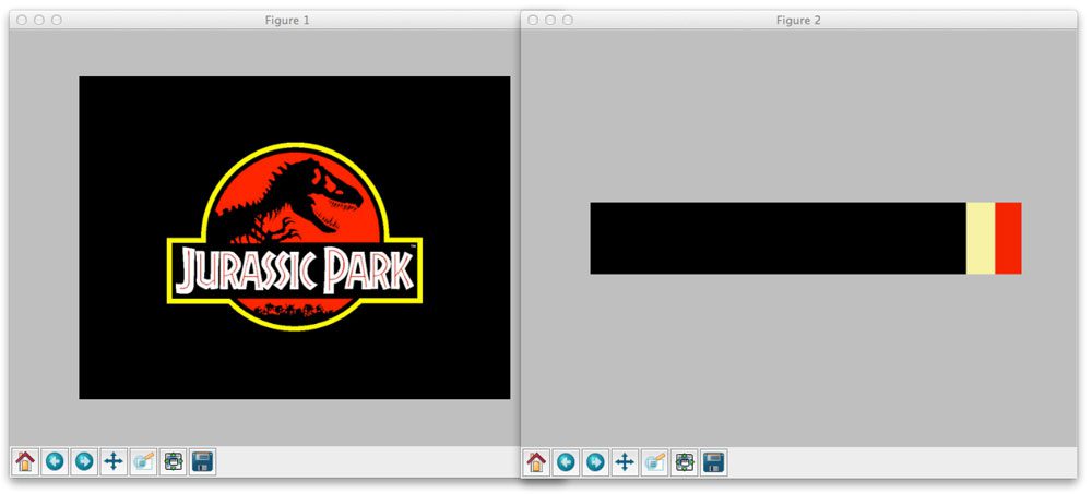
Figure 1: Using Python, OpenCV, and k-means to find the most dominant colors in our image.
Here you can see that our script generated three clusters (since we specified three clusters in the command line argument). The most dominant clusters are black, yellow, and red, which are all heavily represented in the Jurassic Park movie poster.
Let’s apply this to a screenshot of The Matrix:
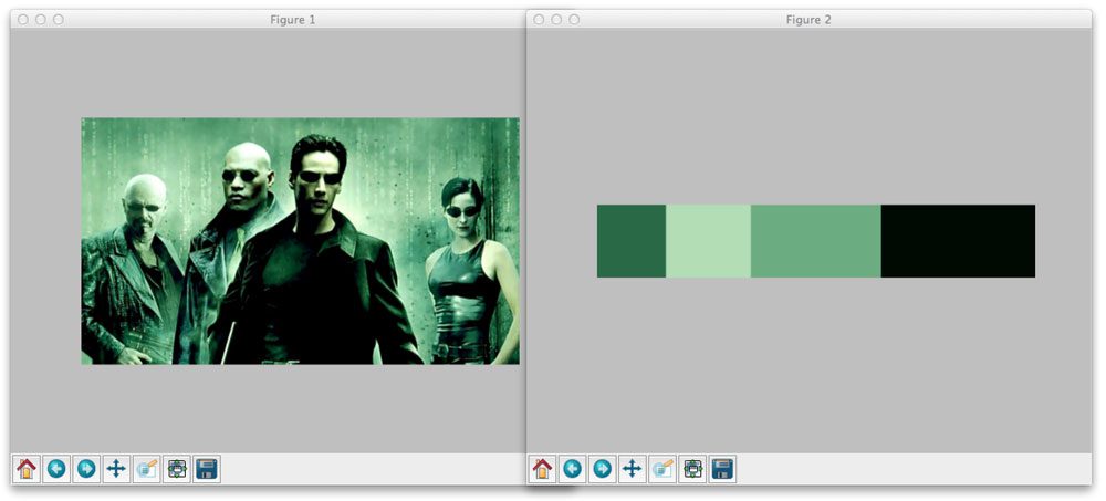
Figure 2: Finding the four most dominant colors using k-means in our The Matrix image.
This time we told k-means to generate four clusters. As you can see, black and various shades of green are the most dominant colors in the image.
Finally, let’s generate five color clusters for this Batman image:

Figure 3: Applying OpenCV and k-means clustering to find the five most dominant colors in a RGB image.
So there you have it.
Using OpenCV, Python, and k-means to cluster RGB pixel intensities to find the most dominant colors in the image is actually quite simple. Scikit-learn takes care of all the heavy lifting for us. Most of the code in this post was used to glue all the pieces together.

Course information: 25 total classes • 37h 19m video • Last updated: 7/2021
★★★★★ 4.84 (128 Ratings) • 10,597 Students Enrolled
I strongly believe that if you had the right teacher you could master computer vision and deep learning.
Do you think learning computer vision and deep learning has to be time-consuming, overwhelming, and complicated? Or has to involve complex mathematics and equations? Or requires a degree in computer science?
That’s not the case.
All you need to master computer vision and deep learning is for someone to explain things to you in simple, intuitive terms. And that’s exactly what I do. My mission is to change education and how complex Artificial Intelligence topics are taught.
If you're serious about learning computer vision, your next stop should be PyImageSearch University, the most comprehensive computer vision, deep learning, and OpenCV course online today. Here you’ll learn how to successfully and confidently apply computer vision to your work, research, and projects. Join me in computer vision mastery.
Inside PyImageSearch University you'll find:
- ✓ 25 courses on essential computer vision, deep learning, and OpenCV topics
- ✓ 25 Certificates of Completion
- ✓ 37h 19m on-demand video
- ✓ Brand new courses released every month, ensuring you can keep up with state-of-the-art techniques
- ✓ Pre-configured Jupyter Notebooks in Google Colab
- ✓ Run all code examples in your web browser — works on Windows, macOS, and Linux (no dev environment configuration required!)
- ✓ Access to centralized code repos for all 400+ tutorials on PyImageSearch
- ✓ Easy one-click downloads for code, datasets, pre-trained models, etc.
- ✓ Access on mobile, laptop, desktop, etc.
Click here to join PyImageSearch University
Summary
In this blog post I showed you how to use OpenCV, Python, and k-means to find the most dominant colors in the image.
K-means is a clustering algorithm that generates k clusters based on n data points. The number of clusters k must be specified ahead of time. Although algorithms exist that can find an optimal value of k, they are outside the scope of this blog post.
In order to find the most dominant colors in our image, we treated our pixels as the data points and then applied k-means to cluster them.
We used the scikit-learn implementation of k-means to avoid having to re-implement it.
I encourage you to apply k-means clustering to our own images. In general, you’ll find that smaller number of clusters (k <= 5) will give the best results.

Enter your email address below to get a .zip of the code and a FREE 17-page Resource Guide on Computer Vision, OpenCV, and Deep Learning. Inside you'll find my hand-picked tutorials, books, courses, and libraries to help you master CV and DL!