Trusting the Untestable: Validation and Diagnostics for the Doubly Robust Models

Sitemap

[

Lyft Engineering

](https://eng.lyft.com/?source=post_page---publication_nav-25cd379abb8-00853df009df---------------------------------------)

[

](https://eng.lyft.com/?source=post_page---post_publication_sidebar-25cd379abb8-00853df009df---------------------------------------)

Stories from Lyft Engineering.

written by Ross Chu and Shima Nassiri

The Causal Frontier: Measurement Beyond Randomization

The gold standard for determining the causal impact of a policy or product change at a company like Lyft is the A/B test (randomized experiment). By randomly assigning users to a treatment or control group, A/B tests inherently eliminate bias, providing clean estimates of the Average Treatment Effect (ATE). However, many critical business questions and large-scale initiatives simply cannot be randomized. This forces scientists to move past traditional experimentation and leverage quasi-experimental methods.

We rely on non-randomized measurement in several key scenarios across Lyft:

• Partnerships and Policies: Assessing the incremental impact of a partnership (e.g., linking two company accounts) is often a non-randomized assignment. Since these collaborations require coordinated operational work across both companies and are typically announced or promoted broadly, this makes controlled randomization impractical.
• Long-Term Effect (LTE): Measuring effects that unfold over a long period, like the LTE of high prices on future rides, is typically handled by observational studies.
• Post-Launch Evaluation: Continuous monitoring of a policy after it has been fully rolled out requires a method that doesn’t involve costly holdout groups or degradation tests.
• Biased Data: In cases where pre-existing experimental data is found to have an imbalance, a quasi-experimental approach can potentially leverage the biased data instead of requiring a costly rerun.

Introducing Doubly Robust Models: Causal Inference Without Randomness

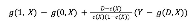
To address these non-randomized measurement needs, Lyft relies on various quasi-experiment estimators. In this blog we specifically focus on using the Augmented Inverse Propensity Weighting (AIPW) model. This model was first established at Lyft to measure the impact of a negative user experience on future topline metrics like rides and bookings; AIPW is a form of doubly robust estimation used to estimate the Average Treatment Effect (ATE) or Average Treatment Effect on Treated (ATT).

The doubly robust nature is what makes the AIPW model so powerful: the formula relies on fitting two separate models for a given set of confounders X and treatment D — the outcome model, g(D, X), and the propensity score model, e(X) — and the overall estimator consistently estimates the true ATE if at least one of these two models is correctly specified.

The Critical Need for Validation

Unlike A/B tests, quasi-experiments lack the fundamental guarantee of unbiasedness provided by randomization. This makes validation, diagnostics, and trust-building absolutely critical. If we cannot randomize the treatment assignment, we must rely on a large set of control variables (confounders) to adjust for pre-exposure differences between the treatment and control groups. This adjustment process makes the analysis highly susceptible to bias if not correctly executed and rigorously checked. The core validation pillars are centered on managing confounders and monitoring model diagnostics, as we’ll explore in the next section.

The Validation Engine: Confounders and Diagnostics

Since quasi-experiments lack the inherent randomization of A/B tests, we must prove the validity of our causal estimates through rigorous inputs and explicit model diagnostics. We build trust in every single result through Confounder Management and a Diagnostic Scorecard.

1. Rigorous Data and Confounder Inputs

The greatest threat to a quasi-experiment’s validity is selection bias — users with certain characters are more likely to be treated by the policy, making the control group not a proper counterfactual for the treatment group. The only way to correct for this is by meticulously identifying and controlling for these pre-existing differences, known as confounders. At Lyft, we have developed a quasi-experimentation platform that makes this process mandatory and customizable.

a) The Confounder Set Requirement

The analysis requires potentially hundreds of features/confounders to adequately reduce bias. The quasi-experimentation platform doesn’t allow users to skip this step; users are required to select or define one confounder set for AIPW analysis.

• Pre-defined sets: Users can choose from established sets on the platform that are pre-defined as SQL queries to pull the relevant data.
• Customization is key: Crucially, the platform exposes the underlying SQL query, allowing users to customize, modify, add, or remove variables within a set to perfectly match their specific use case.
• Preventing leakage: The system automatically ensures confounder data is gathered from before the user’s first exposure date to the treatment, preventing leaky covariates that would incorrectly attribute the treatment’s effect to a non-causal variable.

b) The Balancing Act: Correcting for Downsampling Bias

A core task in data preparation for AIPW is balancing the size of the treatment and control groups in the presence of imbalance data. When the one group is smaller than the other, the system randomly downsamples the larger group to achieve balance. However, this random downsampling introduces a new scientific challenge:

• Non-Representative Samples: Even if the original sample satisfies model assumptions across treatment groups, taking a random subset of the larger group may make that subset non-representative of the true population distribution with respect to the confounders.

To recover the true population-level ATE, we apply a correction in the AIPW estimates per Ballinari (2024), which involves two related concepts:

i. Propensity Score Correction: We must convert the sample-estimated propensity score, p_s(X), back into the true population propensity score, p(X), using a conversion formula that accounts for the downsampling ratio L. This ensures the model uses the real probability of being treated in the population, not just in the sample.

ii. Outcome Reweighting: After the propensity score correction, the efficient scores must be subjected to a weighted average based on the sampling ratio. Specifically, for every observation in the downsampled control group, we must account for the fact that it represents 1/L copies of the original population. This process involves uniformly rescaling the weights of each observation so they average to 1.

This reweighting of outcomes is a critical scientific refinement currently being implemented to debias the results and ensure the final ATE estimate accurately reflects the total impact on the original population.

2. Model Diagnostics and Assumptions

The output of every AIPW analysis on our quasi experimentation platform is a scorecard with two essential tabs: the Scores Tab and the Diagnostic Tab. The Diagnostic Tab is where we evaluate the model’s health to look for clues that its fundamental assumptions hold, providing visual proof of the estimation quality. Below are two of the tens of diagnostics we show users:

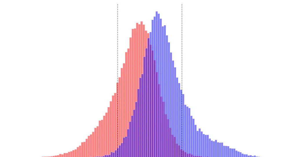
i. Checking Common Support (Propensity Overlap)

Get Shima Nassiri’s stories in your inbox

Join Medium for free to get updates from this writer.

The AIPW model relies on the common support assumption (or overlapping assumption), meaning that for any given set of confounders, there must be a non-zero probability of being in either the treatment or control group (0<e(X)<1). If this assumption is violated, the inverse propensity score weights explode. This means that the outliers will receive an extreme weight and take over the overall effect.

The platform provides a histogram visualizing the Propensity Overlap between the control and treatment groups. Below are examples of sufficient and insufficient overlaps between treated and control groups

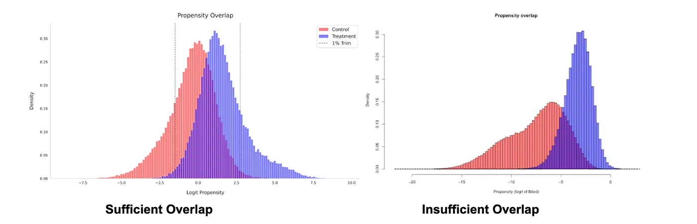
If the overlap is poor, the causal estimates are unreliable. The analysis is further refined by applying a user-defined trim level to discard extreme propensity score values and satisfy the common support assumption.

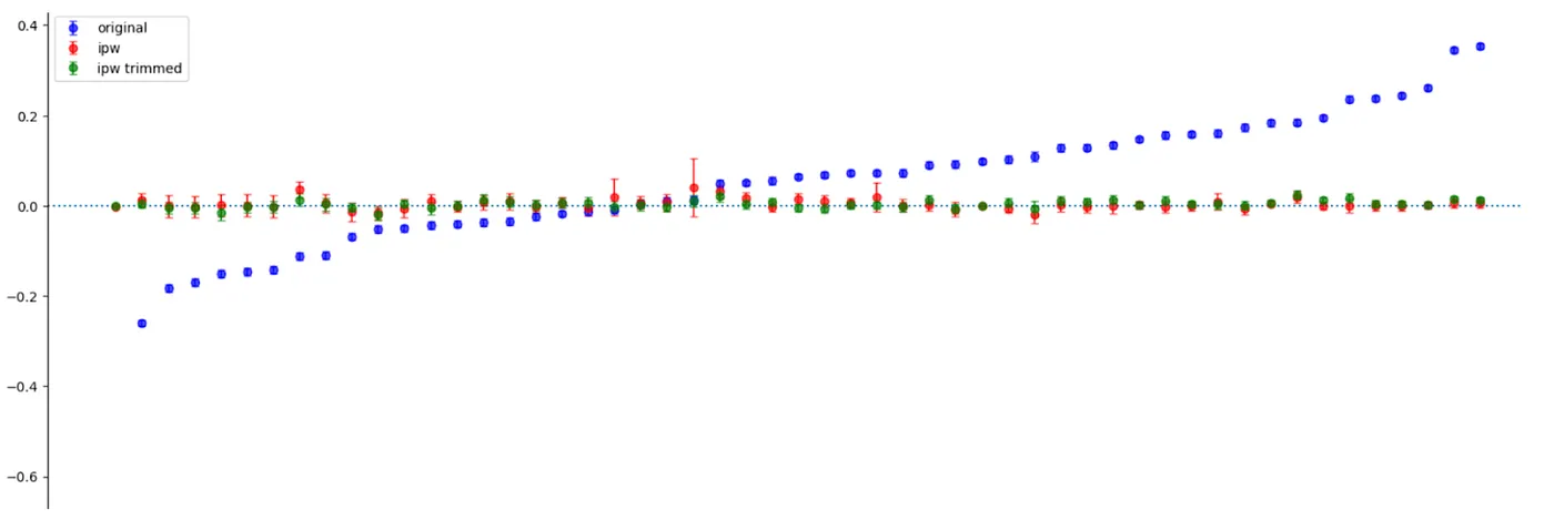
ii. Ensuring Covariate Balance

The primary goal of using confounders is to achieve a state where the treatment and control groups are statistically similar on all observed characteristics.

A key diagnostic graph illustrates the Covariate Balance before and after adjustment.

• Before Adjustment (Original): Shows the initial difference (bias) in each feature between the groups.
• After Adjustment (IPW/IPW Trimmed): Shows how well the model has reduced the difference. Successful adjustment moves the metrics close to the dotted zero line, confirming that the confounders are properly balanced.

Measuring Bias in AIPW

Since AIPW is a new addition to our causal inference platform, we needed to verify its performance. We decided to use randomized experiments as our “ground truth” to see how closely our observational AIPW estimates matched experimental results. We looked for an empirical setting where there was both experimental and observational data for the same intervention, time period, and regional markets. This allows us to compare experimental results directly against AIPW estimates derived from observational data, where we controlled for biases using a large set of confounders.

Empirical Setting: Weekly Ride Challenges

Weekly ride challenges are conditional bonuses given to drivers if they complete a certain number of rides within a week. Since these bonus payments are costly, Lyft uses an algorithm to target ride challenges efficiently given a fixed budget. Specifically, the algorithm allocates ride challenges to drivers who are expected to be most responsive. AIPW estimates the effect of ride challenges using observational data by comparing drivers who do versus do not receive the challenges (within the targeted group) while having similar propensity scores.

The experimental ground truth leverages an ongoing experiment to evaluate the effectiveness of ride challenges. In this holdout experiment, drivers are randomly assigned into a “control” group that will not receive a ride challenge. Remaining drivers in the “targeted” group may or may not receive a ride challenge depending on whether they are targeted by the algorithm (illustrated below). AIPW estimates the treatment effect on observational data by comparing drivers who do versus do not receive the challenge within the targeted group.

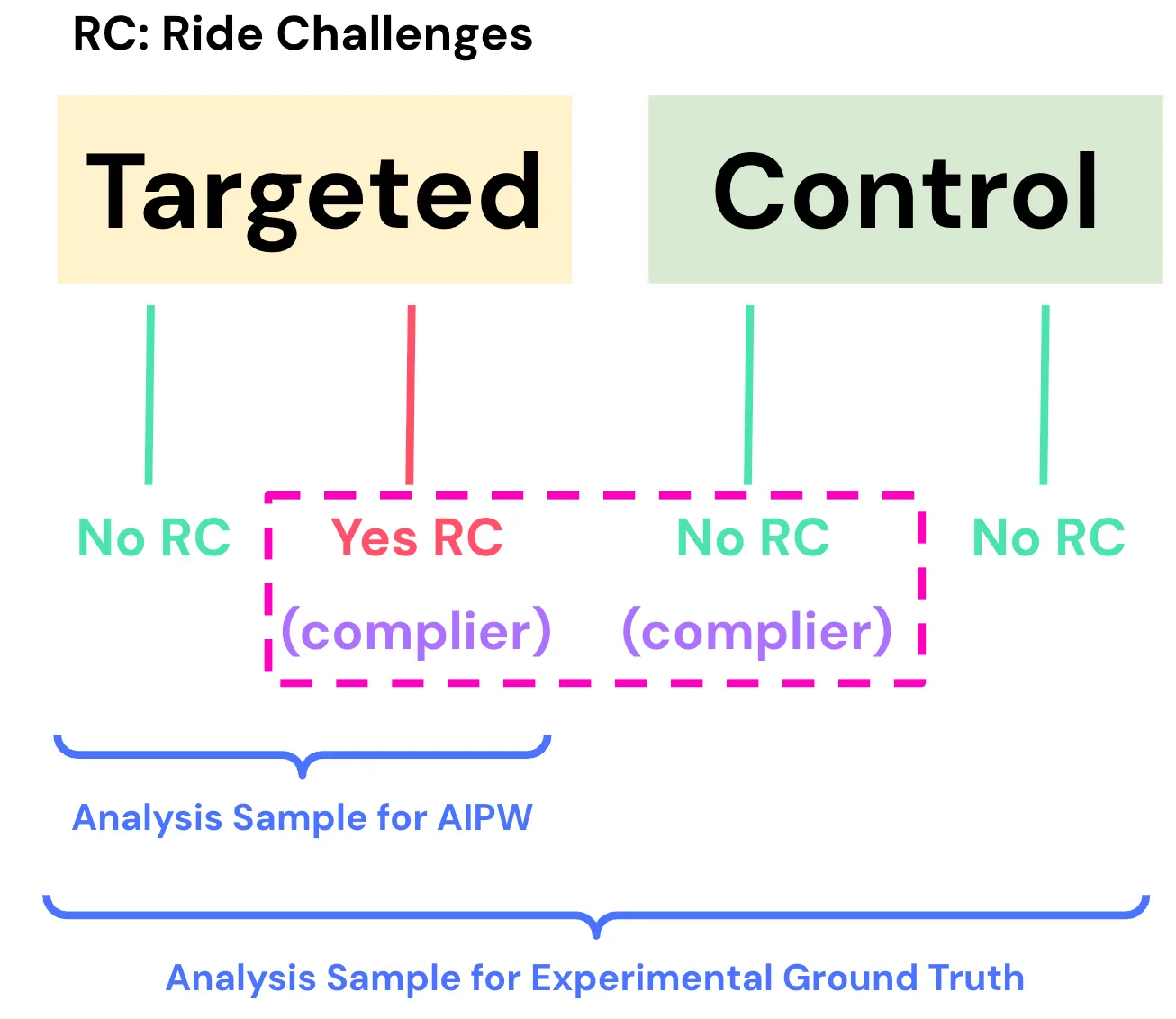
For the experimental ground truth, we cannot directly compare drivers in targeted versus control groups. This is because many drivers in the targeted group do not receive the ride challenge, so a direct comparison would yield unbiased estimates for “potentially” being exposed to ride challenges. This diluted effect would not be comparable with AIPW, which is comparing drivers with versus without the ride challenge.

To get around this issue, we used instrumental variables (IV) to estimate the Local Average Treatment Effect (LATE). Randomized assignment into targeted versus control groups is the “instrument” that influences whether the driver receives the ride challenge, but it does not perfectly determine it. LATE is the treatment effect of ride challenges for “compliers”: drivers who receive the challenge if assigned to the targeted group, and drivers in the control group who would have received the ride challenge if they had been assigned to the targeted group. Conceptually, compliers are “potential targets” who would be targeted by the algorithm for ride challenges, so whether they receive the challenge is solely determined by random assignment into targeted versus control groups. We compare LATE from experimental data with Average Treatment Effect for Treated units (ATET) from observational data, since they both correspond to the effect of ride challenges for drivers who are targeted by the algorithm.

What We Found

Through this careful “apples-to-apples” comparison, we found that AIPW estimates obtained from observational data understate ground truth magnitudes obtained from experimental data through IV estimates. In the first row of the table below, AIPW estimates that ride challenges increase driver hours by 11.1%, while the experimental estimate suggests a 13.3% effect. ==The AIPW estimate is 2.1 percentage points below the experimental estimate, or equivalently, 16.2% lower than the ground truth magnitude.==

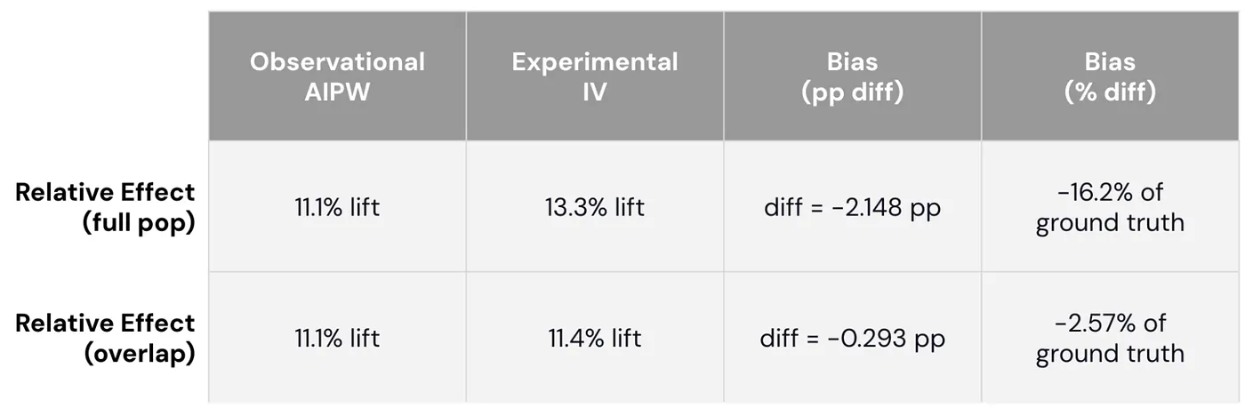
To understand the root cause, we explored whether this discrepancy is because the analysis sample for AIPW is different from the overall population. Since AIPW requires the same propensity score values to be observed in treated and control groups, the analysis sample trims out drivers whose propensity scores are too high or too low. Since this is a subset of the overall population, the discrepancy observed earlier may reflect differences in the populations they represent.

To test this hypothesis, we used the propensity score model to find a comparable subset in the experimental data with the same range of hypothetical propensity scores. The second row of the table shows that the discrepancy between observational AIPW and experimental IV is minimal when comparing within this subset. The estimated effect from AIPW is only -0.3 percentage points below the experimental ground truth (smaller by 2.57%). This large reduction in discrepancy shows that AIPW understates the ground truth primarily because the trimmed analysis sample is different from the overall population.

However, this doesn’t mean that AIPW will always understate the experimental ground truth. In fact, there is a well-known study at Facebook that actually found the opposite. Whether AIPW understates or overstates the true effect heavily depends on the empirical context. In our case, ride challenges are targeted to the most effective drivers, who tend to have higher propensity scores. It is difficult to find drivers who have similar propensity scores but did not receive the ride challenge, since most of them are targeted by the algorithm. ==As a result, the most effective drivers in the treated group end up being trimmed out of the analysis sample due to a lack of comparable drivers in the control group.== Since AIPW estimates the treatment effect on an analysis sample that excludes the most effective drivers, it makes sense that AIPW understates the true effect on the overall population that includes such drivers.

Improving the AIPW Platform Through our Learnings

To summarize our findings, we initially found that the estimated effect from AIPW understates the experimental ground truth. A deep dive revealed two key drivers:

1. Hidden Confounders: Even with a rich feature set, hidden confounders can still bias estimates.
2. Propensity Trimming: Trimming users with extreme propensity scores (to satisfy the common support assumption) shifted our analysis sample so it was no longer representative of the target population.

This discrepancy disappeared once we subset the experimental data to match the analysis sample in AIPW. The “bias” was largely due to measuring the effect on a narrower segment of users who behaved differently than the general population.

Unobserved confounding and trimming on propensity scores can be more problematic in some applications than others. Since AIPW is not reliable when these issues are severe, we introduced two additional diagnostics to recognize when our estimates are vulnerable to these issues:

• Marginal Sensitivity Model (Zhao et al., 2018): This metric quantifies the robustness of estimates to hidden confounders, which bias our propensity scores. It measures the required discrepancy between true and estimated propensities to change our directional conclusions. More specifically, the discrepancy factor G quantifies the extent to which true versus observed odds ratios diverge due to unobserved confounding (1/G ≤ odds ratio ≤ G). This is used to infer bounds on true propensity scores given observed propensities e(X) and factor . We use this to construct worst-case bounds on treatment effects, and the diagnostic metric is the smallest value so that the worst case bounds touch zero. Higher values for this sensitivity metric indicate that the direction of true impact does not change even with large discrepancies in propensity scores due to unobserved confounding.
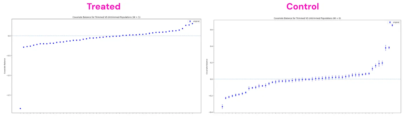
• Covariate Comparisons for Trimmed vs. Untrimmed: We plot observed characteristics of trimmed users against untrimmed users. If trimmed users look significantly different from untrimmed users, then our analysis sample would lack external validity to the overall population. Each point below reports the normalized difference between trimmed versus untrimmed users for each observed covariate, separately for treated and control groups. In the example below, users with certain characteristics are more likely to be trimmed in the treated group than they are in the control group. If users with certain characteristics are more likely to be trimmed, then the estimated ATE from the analysis sample may overstate or understate the true ATE in the overall population.

Conclusion: Trustworthy Causal Impact at Scale

Integrating AIPW into our platform has unlocked the ability to measure causal impact when A/B tests are infeasible. Since quasi-experimentation platform is a new capability at Lyft, we needed to rigorously validate the model to build stakeholders’ trust around the tool. Validation will continue to be essential as we onboard additional tools to the platform, which will help us deliver trustworthy insights for our most complex challenges at Lyft’s marketplace.

Lyft is hiring! If you’re passionate about experimentation and measurement, visit Lyft Careers to see our openings.

Responses (3)Write a response

[

What are your thoughts?

](https://medium.com/m/signin?operation=register&redirect=https%3A%2F%2Feng.lyft.com%2Ftrusting-the-untestable-validation-and-diagnostics-for-the-doubly-robust-models-00853df009df&source=---post_responses--00853df009df---------------------respond_sidebar------------------)

This was a great read. I learned a ton! Thank you for sharing your experience!

[

](https://medium.com/m/signin?actionUrl=https%3A%2F%2Fmedium.com%2F_%2Fvote%2Fp%2F2bdab8f879e5&operation=register&redirect=https%3A%2F%2Fmedium.com%2F%40elashrry%2Fthis-was-a-great-read-i-learned-a-ton-thank-you-for-sharing-your-experience-2bdab8f879e5&user=Ahmed+Elashry&userId=455c18d72dfb&source=---post_responses--2bdab8f879e5----0-----------------respond_sidebar------------------)

==The AIPW estimate is 2.1 percentage points below the experimental estimate, or equivalently, 16.2% lower than the ground truth magnitude.==

An interesting score that I would have loved to see is the overlap percentage of confidence intervals, because a lift in the experiment is not a "ground truth''.

[

](https://medium.com/m/signin?actionUrl=https%3A%2F%2Fmedium.com%2F_%2Fvote%2Fp%2Fd33b6ca77faa&operation=register&redirect=https%3A%2F%2Fmedium.com%2F%40elashrry%2Fan-interesting-score-that-i-would-have-loved-to-see-is-the-overlap-percentage-of-confidence-d33b6ca77faa&user=Ahmed+Elashry&userId=455c18d72dfb&source=---post_responses--d33b6ca77faa----1-----------------respond_sidebar------------------)

==As a result, the most effective drivers in the treated group end up being trimmed out of the analysis sample due to a lack of comparable drivers in the control group.==

To make it precise, and correct me if I am wrong.Here we are talking about the sample for the AIPW analysis, i.e. the randomised treated group. Then the most effective drivers in the RC are trimmed out due to a lack of comparable drivers in the No…more

[

](https://medium.com/m/signin?actionUrl=https%3A%2F%2Fmedium.com%2F_%2Fvote%2Fp%2Fa81756189630&operation=register&redirect=https%3A%2F%2Fmedium.com%2F%40elashrry%2Fto-make-it-precise-and-correct-me-if-i-am-wrong-a81756189630&user=Ahmed+Elashry&userId=455c18d72dfb&source=---post_responses--a81756189630----2-----------------respond_sidebar------------------)