Real-Time Spatial Temporal Forecasting @ Lyft

Real-time spatial temporal forecasting is often used to predict market signals, ranging from a few minutes to a couple of hours, at fine spatial and temporal granularity. For example, we can predict rideshare demand and supply at geohash-6 level for every 5 minute interval in the next hour for an entire city or region. The forecast also runs at a high frequency (e.g. every minute) with real-time input of the most refreshed data to capture the latest marketplace conditions in fine detail, including local spikes and dips.

Lyft currently operates in hundreds of North American cities and regions. Our spatial temporal forecasting models predict forecast values for 4M geohashes per minute, per signal.

Use Cases

Predictions from real-time forecasting are often used for inputs into levers that balance real-time demand and supply across space. For example:

• Dynamic pricing: As a platform, maintaining marketplace balance is one of Lyft’s top missions. Dynamic pricing maintains balance in real-time by raising prices to dampen demand when drivers are scarce and lowering prices to encourage rides when there are more drivers.
• Real-time driver incentives: In contrast to dynamic pricing managing demand, real-time driver incentives achieve marketplace balance by raising drivers’ earnings to attract drivers to come online during undersupply or relocate from oversupplied to undersupplied areas. Similarly, understanding the current and near-future marketplace conditions in different locations is essential to the incentive model.

Challenges

The high dimension, high frequency nature of real-time spatial temporal forecasting presents unique challenges compared to low dimension, low frequency time series forecasting.

Large Computation Restricts Practical Model Choices and System Design

More computation power is needed for heavy spatial and temporal data processing and fast online inference, which can restrict our model choices and system design in practice. Large complex models, such as deep neural networks, might give more accurate forecasts in theory, but they also cost more to run, take longer, and can be harder to keep stable and scale up. This can cancel out the accuracy gains.

Noisy Signals Reduce Forecasting Accuracy

When analyzing signals with greater spatial and temporal detail, such as minutely geohash-6 level rideshare demand and supply, they can become noisier compared to when viewed at a more aggregated level. Specifically, we observe:

• Sparser signals with many zero observations;
• Increase in intermittent local spikes and dips, usually lasting from a few minutes to about 30 minutes.

These local fluctuations are often due to events like concerts, sports, and community gatherings, which may not be noticeable at broader hourly, daily, or regional levels, but become significant when viewed in detail.

Modeling such impact can be challenging for multiple reasons:

• Data availability & accuracy: Getting comprehensive event data can be costly in practice. Even with access to events data, it can be hard to predict key information such as event end time or impact time at the desired accuracy level. For example, although an American football game displays 5 minutes left on the screen, the actual event end time can vary from 5 to 30 minutes.
• Compound effect: In our experience, the actual impact of events on rideshare demand is usually compounded with other factors; for example:
  * Venue operation like shuttle services and designated rideshare pickups can affect both demand and supply spatially.
  * Availability of public transit and parking facilities can affect travelers’ mode choice.
  * Nearby amenities, like restaurants, can affect pre- and post-event activities and travel plans.
  * Time of day, day of week, and seasonality can also affect public transit, venue and business operations, affecting demand patterns.

Due to this “noise”, the spatial and temporal correlation and stability at a detailed level can drop significantly from those at an aggregated level. We will discuss how these changes could affect forecast accuracy in the model performance section.

Forecasting Models

We have explored two distinct sets of models for real-time spatial temporal forecasting: classical time-series models and neural network models. In this section, we introduce a few representative models that we have explored at Lyft and/or have been well studied in research papers. We also compare the model performance in terms of forecast accuracy and engineering cost from our implementation. Note that although it’s mentioned in the introduction that local events can contribute to fluctuations in our signals, we will not explicitly discuss events or events modeling here as it is a complicated topic worth another discussion of its own.

Time Series Models

Some of the time series models we have explored include:

• Linear regression models like auto-regression and ARIMA: These simple time series models use past data (linear combinations or weighted averages) to predict the future. To adapt single time series models on spatial data (multiple correlated time series), we can either assume the same model weights for all regional geohashes or divide the region into partitions based on signal history, assigning specific weights to each partition.
• Spatial temporal covariance models: Instead of treating different geohashes (or partitions) as independent time series, we can estimate and model spatial temporal correlations explicitly (see Chen et al. [2021]).
• Spatial temporal correlation through dimension reduction: Assuming that many geohashes are correlated, we can apply dimension reduction approaches like SVD and PCA to project thousands of time series to a few dozen, with correlation embedded in the dimension reduction process. We then apply traditional time series models on the reduced dimensions for forecasting, and finally project the forecasts back to the original geohash dimension (see Skittides Fruh [2014], Grother & Reiger [2022]).

Neural Net Models

Deep neural network (DNN) models have emerged as powerful alternatives due to their capacity to automatically handle complex non-linear spatial and temporal patterns without extensive feature engineering (Casolaro et al. [2023]; Mojtahedi et al. 2025). Some of the DNNs we tested are:

• Recurrent neural networks (RNN) and variants like long short-term memory (LTSM): He et al [2021], Abduljabbar et al. [2021]. RNNs’ fundamental architecture for sequence modeling is perfect for learning temporal correlation by memory retention from previous time steps. However, standard RNNs suffer from vanishing gradient problems when processing long sequences. LSTM networks address this limitation through gating mechanisms.
• Convolutional neural networks (CNN): Zhang et al. [2016], Guo et al. [2019]. CNNs were initially applied to image processing, and recently have been adapted for spatial temporal modeling, treating signal values at each map timestamp like a snapshot of pixels in an image.

A few other emerging DNN models, which we haven’t tested yet but give similar performance in literature, are:

• Graphic neural networks (GNN): Bui et al. [2022], Geng et al. [2022], Corradini et al. [2024]. GNNs have been well-applied to graph-structured data in applications like behavior detection, traffic control, and molecular structure study, where nodes and edges represent entities and their relationships. In spatial temporal forecasting, it is assumed that the signal value of a node depends on its own history and the history of its neighbors, whose weights are estimated by specific blocks or modules in the GNN structure.
• Transformer models: Wu et al. [2020], Wen et al. [2022]. Inspired by their success in natural language processing, transformer models have been increasingly applied to time series forecasting. However, literature has shown mixed results so far (Zeng et al. [2023]).

Online Implementation & Refitting

Our marketplace is constantly changing from day-to-day and minute-to-minute. In our experience, a model trained on historical data can quickly become obsolete, sometimes in a few days but sometimes in a dozen minutes, in the occurrence of some unknown or unmodeled local events. Therefore, frequently retraining the model is critical to the accuracy of the forecasts. We have implemented the following in our forecasting:

• Refit time series models every minute using the latest observations before running an inference.
  * Due to the simplicity of the model structure and smaller model weights, these models are effortlessly re-trainable without causing significant latency or memory issues.
  * It’s worth noting that some of the time series models, such as those based on dimension reduction, are only partially re-trainable in real-time. While new data samples can update model weights in the reduced dimension, this process requires a longer history, which can be time consuming and can only be completed offline at less frequent intervals.
• Refit DNN models multiple times a day.
  * While theoretically all neural network models can be refitted on new data samples, their model size can cause high latency, making real-time refitting less ideal. Instead, we refit the model separately offline multiple times daily using recent data batches.

Model Performance

In our experience, model choice is a trade-off between forecast accuracy and engineering cost. In this section, we share some learnings from our testing and implementation of time series and DNN models. For those interested in or familiar with forecasting modes, the “Accuracy” section offers technical insights into why certain models outperform others. Alternatively, you can focus on the key learnings highlighted in bold.

Accuracy

While most literature finds that DNN models provide better forecast accuracy than classical time series models, we find it to be only partially true. Below are some of our learnings:

DNNs outperform time series without latency consideration

When latency is not considered and forecasts are simulated at the same refitting frequency (from daily, hourly, to minutely), DNN models overall generate more accurate forecasts than classical time series models. However, as the refitting frequency increases, the accuracy gap reduces significantly; and in some cases, time series models can even outperform DNN models.

Time series outperforms DNNs with latency consideration

When considering latency, simulating time series refitted minutely and DNN refitted hourly results in time series models having better overall accuracy than DNN. Specifically,

1. Time series models are more accurate for forecasting short-term horizons, such as the next 5 to 30 or 45 minutes. In contrast, DNN models can outperform time series in longer horizons, beyond 30 or 45 minutes. Our real-time signal has strong near-term autocorrelation. In other words, what will happen in the next 5 minutes can be similar to what happened in the past 5 minutes; hence, even a simple autocorrelation model can generate a good forecast.This is also true during temporal local spikes caused by irregular events. To illustrate, imagine riders leaving a concert. Rideshare demand usually spikes up fast, stays high in the first 15–20 minutes, then gradually returns to normal in the next 15–20 minutes. As the peak occurs, refitting an autoregression model can quickly pick up the autocorrelation and update the forecast accordingly. Meanwhile, a local spike can temporarily change the spatial correlation across nearby geohashes, and without refitting, it can throw off the forecasts of a DNN model’s estimation of spatial correlation.

   As the forecast moves to a longer horizon, the near-term autocorrelation gets weaker. In the concert example above, a demand spike in the past 5 minutes does not guarantee a spike in an hour. Instead, factors like seasonality, trend, and spatial correlation become more important predictors, which DNN models seem to capture better than classical time series models.

2. Between demand and supply signals, both time series and DNN models tend to give better accuracy on supply; however, time series models are more likely to outperform DNN on demand signals. The rationale behind this is due to different levels of signal noise. Drivers tend to stay online for a while after logging on, resulting in smoother supply patterns than for demand, with less temporary spikes or dips. As a result, supply signals have more stable spatial and temporal correlations, making both sets of models perform better. Meanwhile, riders make on-demand requests based on their individual schedules, which tends to cause more fluctuations in demand pattern, making time series with fast refitting a better option.

   In general, the underlying signal generation process influences the spatial temporal correlation and stability, affecting forecast accuracy. For example, average traffic speed in different locations of a city resembles a Gaussian process, and hence is likely to have a much stronger spatial correlation and more stable temporal pattern compared to a demand signal from a Poisson process.

3. For regions with complicated terrain structures (like lots of hills and lakes), DNN models tend to perform worse than time series models.
   Our conjecture is that complicated terrain structures can weaken spatial correlation; hence, making some of the DNN models less powerful. For example, a city with many mountains and waters can have more pockets with zero demand and supply; and a city with many venues for irregular events can cause more local spikes and dips.

From our learnings, we can conclude that forecast accuracy is heavily dependent on the signal characteristics. Before choosing your model, you should evaluate signals for their spatial and temporal correlation and stability.

Engineering Cost

Real-time spatial temporal forecasting is big in size, and requires a large amount of memory and computation power for heavy data processing and fast online inference. Hence, scalability, stability (e.g. low latency), and computation cost affect the final model and system design.

Given the size of the DNN models, it’s no surprise that they are more costly than time series models. In particular:

• Training cost: DNN models require training on GPU, which can be 100x more expensive than classical time series models that train on CPU. For example, training a DNN model on a few weeks of data of a single region can take a couple of hours on a 128GB GPU, while a classical time series model takes less than a minute on an 8GB CPU. These cost differences can be non-trivial when training separate models for hundreds of regions on dozens of signals.
• Engineering reliability: In our experience, DNN models are more prone to issues like training failures, out-of-memory errors, and high latency, incurring higher maintenance costs.
• Forecast interpretability & debuggability: Forecasts from conventional time-series models are usually more interpretable, making it easy to debug performance issues and overwrite forecasts manually if necessary. For example, a time series can be broken down into trend and seasonality, with events and weather impacts added. Each component can be further examined and overwritten if expert knowledge or external data provides a different projection.

Forecasting Architecture & Tech Stack

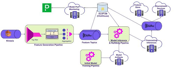
Figure 1: Architecture diagram for forecasting pipelines

The current architecture uses the following technology stack:

Execution flow

1. Before we can run any online inference, an offline model training pipeline needs to be executed to construct online model structure and initialize model weights. These are saved into a model artifacts database for online models to access. This pipeline can also be used to retrain model weights at a scheduled frequency or ad-hocly, and push updated weights to the artifacts database.
2. The system gets the data based on analytics events. These events are generated by our services and client apps.
3. The feature generation pipeline aggregates the events (read about them in this blog post) and passes them through Kafka topics.
4. Features are indexed in OLAP DB (ClickHouse) as short-term historical features with a one day TTL.
5. Our forecasting pipeline takes these features from Kafka topics and OLAP DB. This ensures data consistency across different features based on the window end time of those features. We pass them to our forecasting models hosted on Lyft’s Machine Learning Platform (MLP). Our models also use older historical features (days/weeks), refreshed daily via Airflow DAGs.
6. MLP is responsible for model online inference and asynchronously syncing results to a Kafka topic. If online refitting is implemented, our models can refit using the most recent input and adjust their weights before each inference.
7. This topic is subscribed by downstream services (Rider Pricing, Driver Earnings, etc.) who are interested in forecasted values and want to consume them in real-time. Forecasted values are stored in the Feature Store in case users want to consume them in asynchronous fashion.
8. The forecasted values are also indexed in the OLAP DB, so we can calculate and monitor model performance metrics in real-time.

We have chosen an asynchronous design mainly for scaling and performance reasons.

Forecasted Feature Guarantee

It is important that features come with a quality and reliability guarantee, otherwise it would be difficult for our customers to build products with confidence. For each signal, we define a quality guarantee and measure through our internal systems. Specifically, one system generates model performance metrics (e.g. bias, mean absolute percent error) based on the forecasted and historical values stored in the OLAP DB. Another system constantly monitors these metrics, and if the metrics are outside the expected bounds, then it alerts our engineering team.

Conclusion

Forecasting performance is heavily dependent on the characteristics of the forecasted signals, such as spatial temporal granularity, level of noise, spatial temporal correlation, and its stability. In our experience, simple time series models with real-time refitting provide overall better accuracy when the signal is more granular with less stable spatial temporal correlations, and/or when forecasting the near-term horizons. Although a complex DNN model can improve forecasting accuracy if refitted real-time or forecasting for longer horizons, they may not be the best solution for your business due to high computation cost and latency. Businesses often prioritize simpler models with greater interpretability, lower inference latency, a simplified retraining process and, crucially, a lower total cost of ownership. These factors are essential for choosing cost-effective, maintainable solutions in real-world applications.

Acknowledgements

We would like to thank all our forecasting team members (Jim, Glenna, Quinn, Hongru, Bin, Soo, Kyle, Ido, Evan) for their contribution to model and architecture development, as well as the editing team (Jeana) for valuable suggestions and support during writing this blog post.

Want to build ML solutions that impact millions? Join Lyft! We’re leveraging machine learning to solve problems at scale. If you’re passionate about building impactful, real-world applications, explore our openings at Lyft Careers.

Relevant Posts