More efficient multi-vector embeddings with MUVERA

Weaviate 1.31 implements the MUVERA encoding algorithm for multi-vector embeddings. In this blog, we dive the algorithm in detail, including what MUVERA is, how it works, and whether it might make sense for you.

Let's start by reviewing what multi-vector models are, and the challenges that MUVERA looks to solve.

Challenges with multi-vector embeddings​

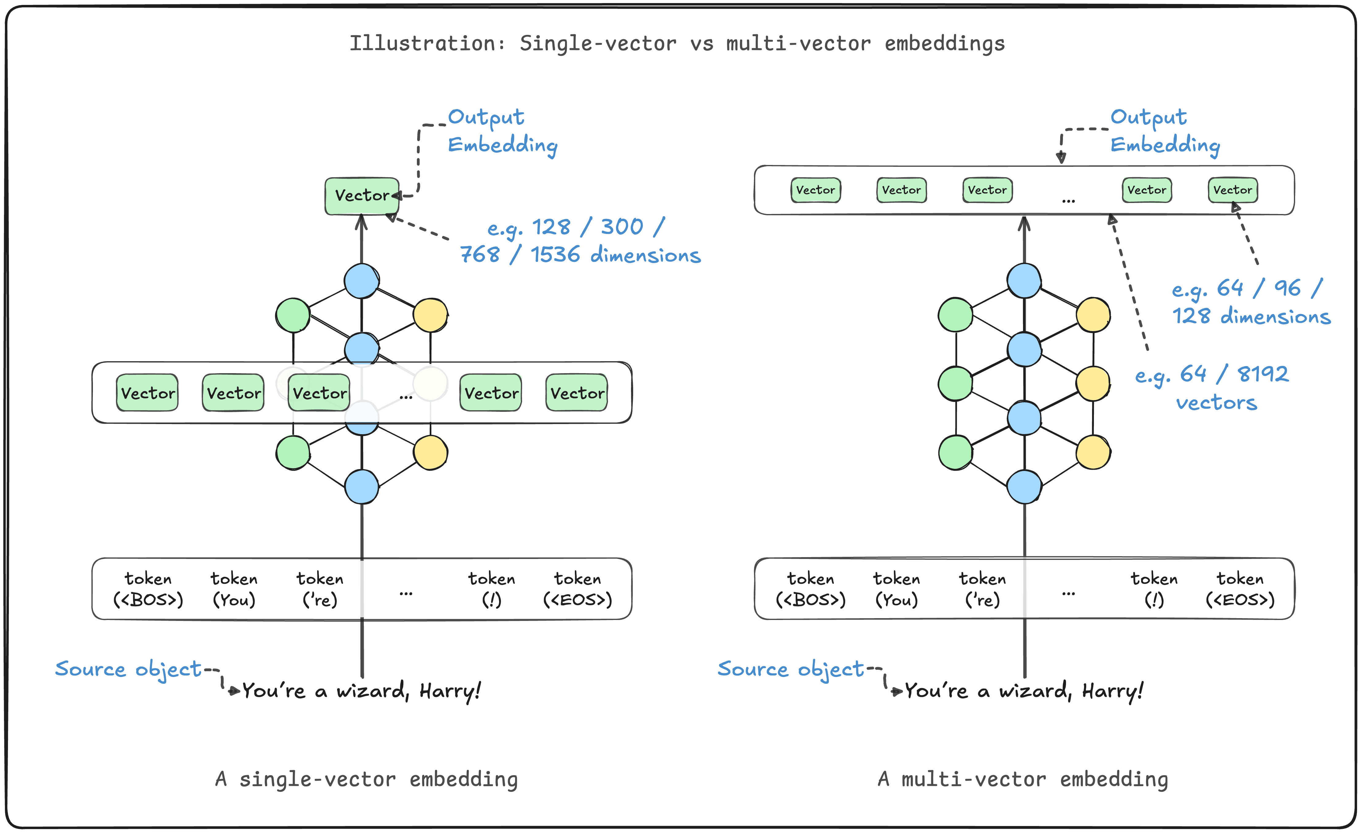
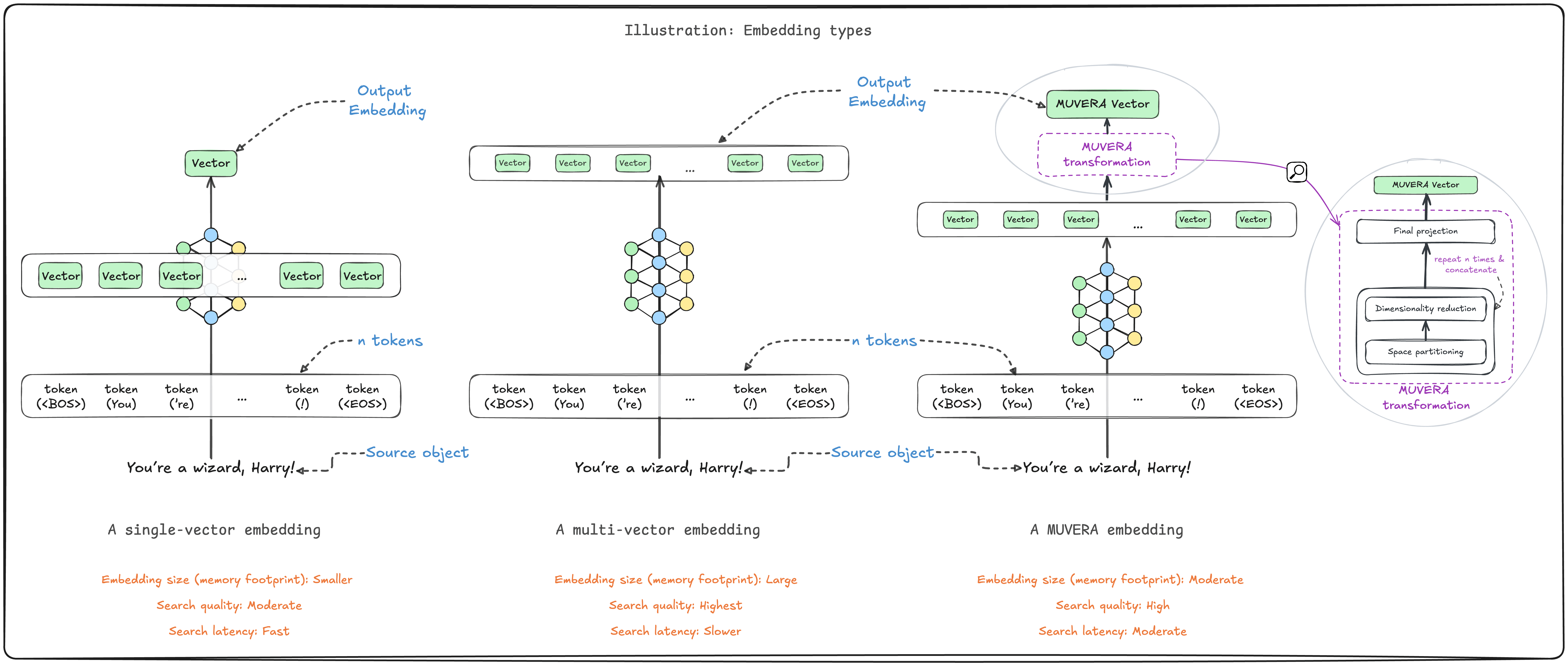
State-of-the-art multi-vector models can dramatically improve retrieval performance by capturing more semantic information than single-vector models. ColBERT models preserve token-level meanings in text, while ColPali/ColQwen models identify and preserve information from different parts of an image, like figures in PDFs as well as textual information.

Single vector to multi-vector comparison

These advantages make multi-vector models a great fit for many use cases. However, multi-vector embeddings carry two potential disadvantages over their single-vector cousins, owing to their size and relative complexity.

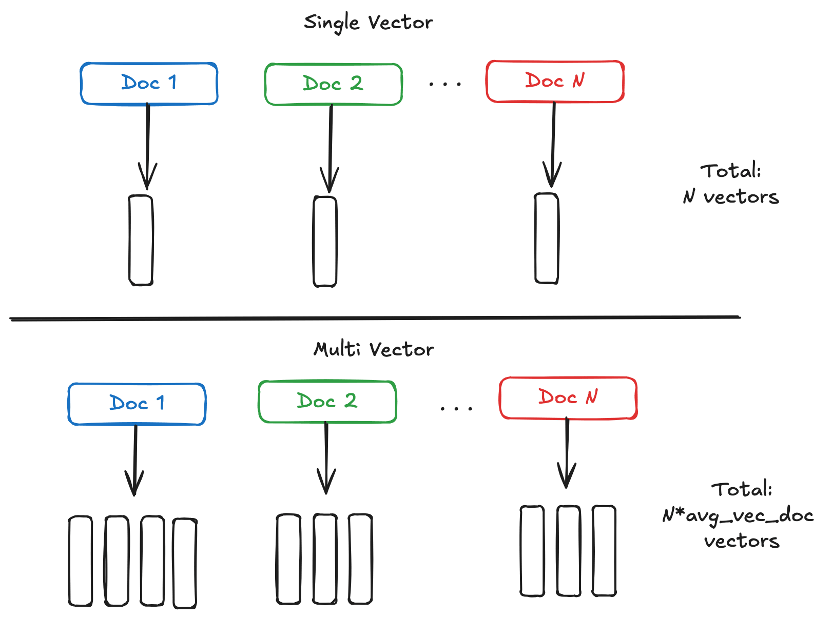
Multi-vector embeddings comprise multiple vectors, each one representing a part of the object, such as a token (text) or a patch (image). Although each vector in a multi-vector embedding is smaller, the whole embedding tends to be larger than a typical single-vector embedding.

Multi-vector embeddings memory comparison

This can lead to a higher memory footprint in use, as many vector search systems use in-memory indexes such as HNSW.

How much larger? Well, as you can see from the image above, the total number of vectors in a multi-vector index will be greater than the single-vector index by average_vectors_per_embedding / (ratio_of_vector_length). As multi-vector embeddings can comprise hundreds up to thousands vectors per document, this can be much larger.

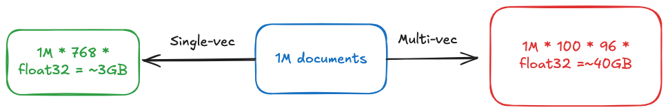
If we embed a million documents of ~100 tokens per document, a single-vector embedding model (of 768 dimensional single-precision, 32-bit, floating point numbers) may require 768 * 1M * 4 bytes = ~3.1GB of memory. On the other hand, a multi-vector embedding model (of 96 dimensions) may require a whopping 96 * 100 * 1M * 4 bytes = ~40GB!

Single vs multi-vector memory usage

And of course, higher memory use also means higher costs, whether it is your own hardware or via cloud infrastructure such as Weaviate Cloud.

Challenge 2: Speed​

A system using multi-vector embeddings can also suffer from slower import and search speeds due to the increased size and complexity.

Vector search involves finding the most relevant embedding(s) from a sea of embeddings. HNSW speeds this up by building a multi-layered graph of vectors to speed up traversing to the right region of vectors and retrieving the right ones.

Multi-vector embeddings introduce additional complexities to this. Multiple vectors must be indexed into the graph per object at ingestion time, and at query time more comparisons are required to retrieve vectors and to calculate their overall similarity.

Given a document embedding D and a query embedding Q, a maxSim operator is typically used to compute the similarity:

sim(D,Q)=∑q∈Qmax⁡d∈Dq⋅dsim(D,Q)=\sum_{q \in Q} \max_{d \in D} q \cdot dsim(D,Q)=q∈Q∑​d∈Dmax​q⋅d

This is a non-linear operation which loops over each query token and compute the similarity between that query token and all the document token choosing the most similar one. In other words, the MaxSim searches the "best-match" for a query term among all the document ones.

While an elegant method, this calculation is another overhead that is unique to multi-vector embeddings.

To improve the performance of multi-vector embeddings, Google's research group proposed MUVERA (Multi-Vector Retrieval via Fixed Dimensional Encodings) which aims to reduce the memory occupancy to store the multi-vector embeddings using fixed encodings.

MUVERA to the rescue​

MUVERA encodes multi-vector embeddings into single vector embeddings by building fixed dimensional encodings (FDE) whose length is independent of the number of vectors in the original multi-vector embedding. This reduces the size of the embedding, and improves efficiency of calculations.

But how does MUVERA do this while minimizing losses in recall?

The key idea​

MUVERA takes as input a multi-vector embedding (DDD) and transforms it into a single-vector embedding (dsingled_{single}dsingle​):

encode(xmulti)  ⟹  xsinglex∈{D,Q}encode(x_{multi})\implies x_{single} \quad \quad x \in \{D, Q\}encode(xmulti​)⟹xsingle​x∈{D,Q}

In order to say if this function is "good enough" we want to maximize the similarity of the two key measures:

• similarity of the encoded embeddings xsinglex_{single}xsingle​ (aka single-vector embedding), and
• similarity of the multi-vector embeddings xmultix_{multi}xmulti​

The more similar these two are, the better that xsinglex_{single}xsingle​ is as an approximation of xmultix_{multi}xmulti​. Ideally, we want:

maxSim(D,Q)≈dsingle⋅qsinglemaxSim(D,Q)\approx d_{single} \cdot q_{single}maxSim(D,Q)≈dsingle​⋅qsingle​

wheredsingle=encode(D)∧qsingle=encode(Q)where \quad d_{single} = encode(D)\quad \land q_{single}=encode(Q)wheredsingle​=encode(D)∧qsingle​=encode(Q)

This transform simplifies the approximate nearest neighbor search problem for multi-vector embeddings to that involving only single vector embeddings.

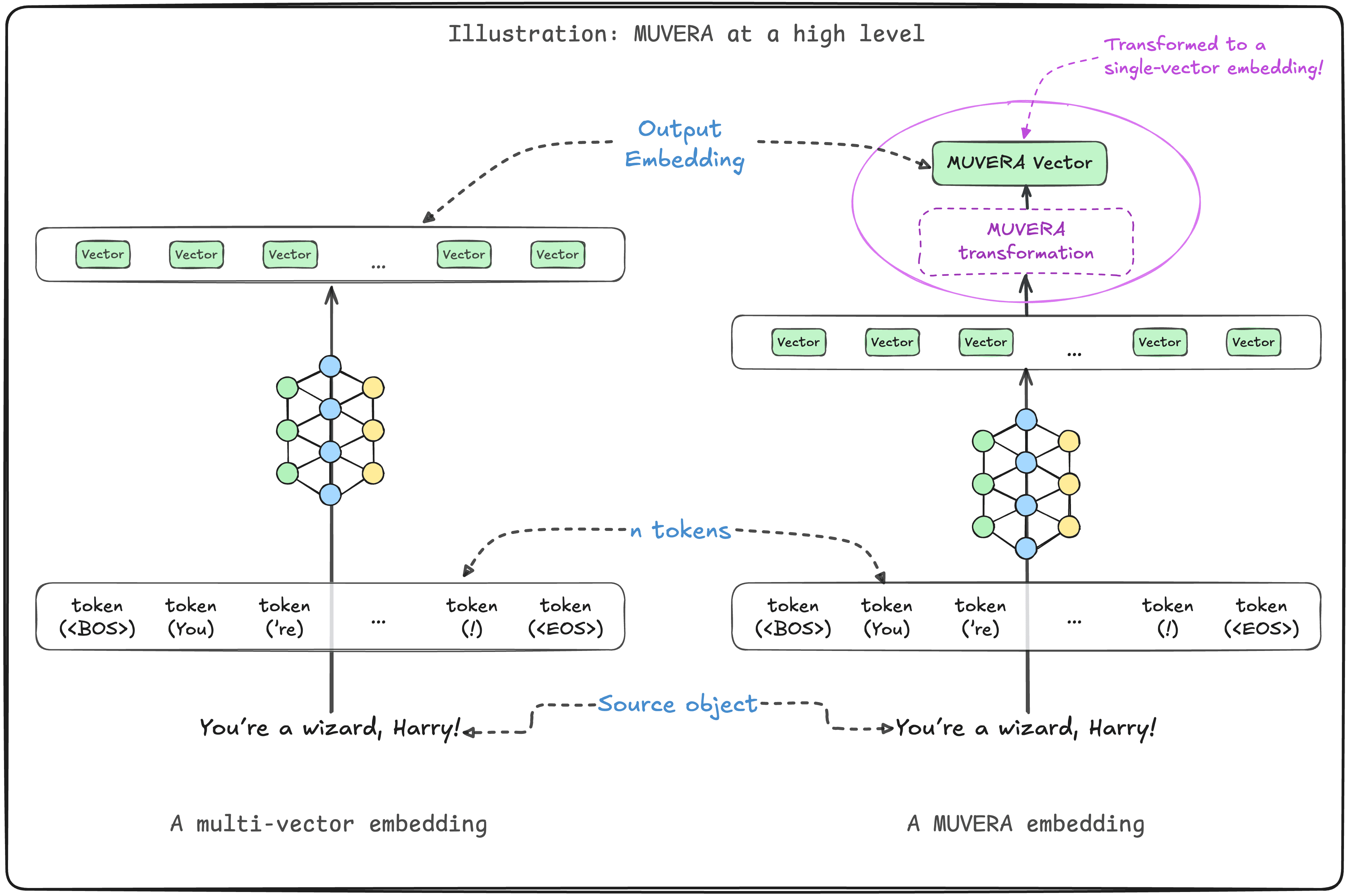
MUVERA high level overview

Recall the above scenario with a million documents and 100 vectors per document. Without the MUVERA encoding we would have 100M vectors to be indexed. Instead, using the FDE vector we will be working with only 1M vectors, leading to an HNSW graph of only 1% of the size!

So how does MUVERA achieve this goal?

How MUVERA works​

Recall that the main goal here is to build an FDE dsingled_{single}dsingle​ which approximates the semantics of the multi-vector embedding DDD.

MUVERA does this in four steps:

1. Space partitioning
2. Dimensionality reduction
3. Multiple repetitions
4. Final projection

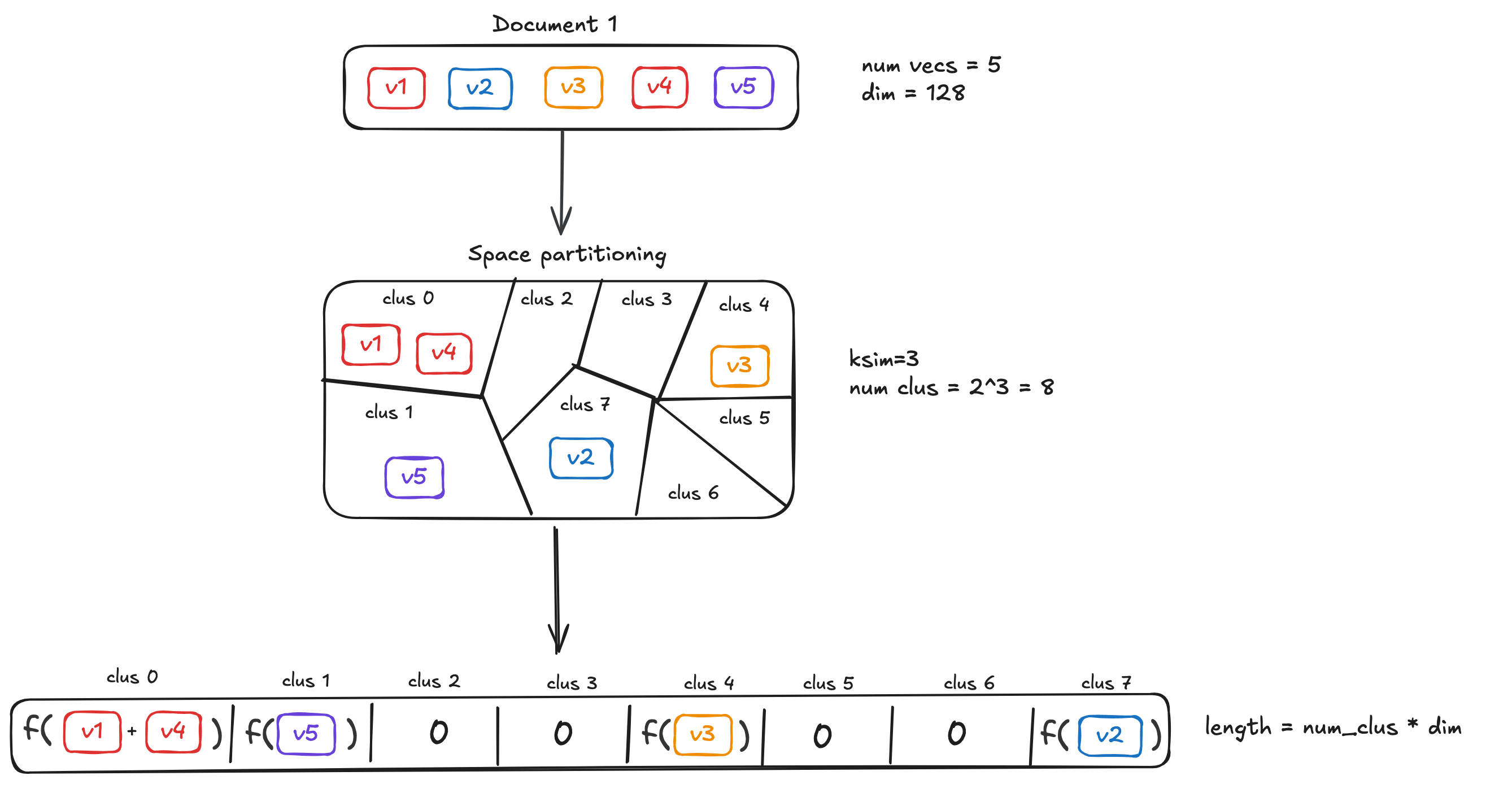
Space partitioning​

The first step consists of partitioning the vector space into BBB "buckets". This can be achieved using k-means clustering or using locally sensitive hashing (LSH) functions.

Ideally, we want a partitioning function φ\varphiφ that given an input vector xxx will return a bucket id k=φ(x)k=\varphi(x)k=φ(x) where k=1,…,Bk=1,\dots,Bk=1,…,B. Here is an illustration, assuming a set of 8 clusters:

MUVERA steps 1

MUVERA steps 2

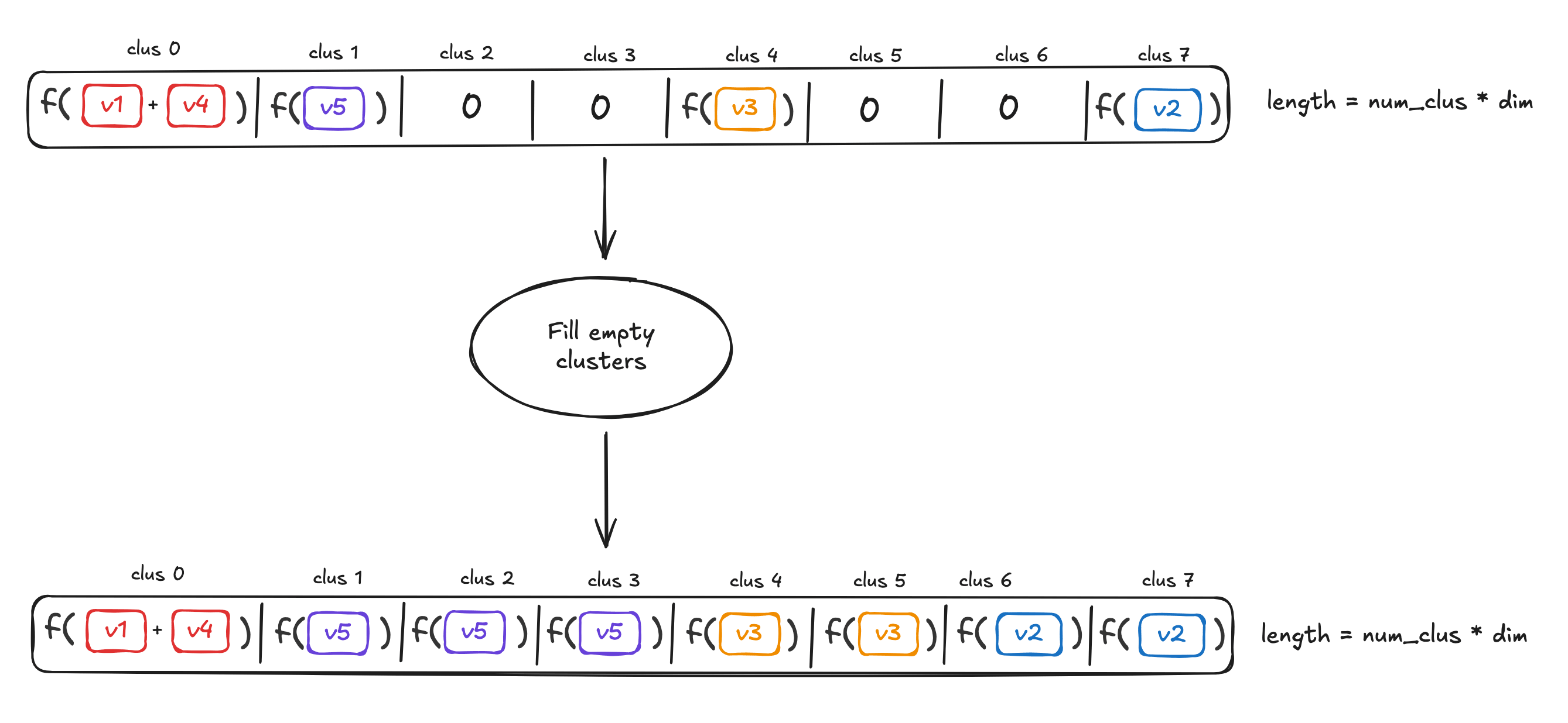
As shown in the figure, each vector is assigned to one of the clusters. Two further calculations are done - one to derive a representative (e.g. average or centroid) sub-vector, and another to fill empty clusters.

Now that the partitioning function is ready, we can create a sub-vector dkd_kdk​ for each bucket k=1,…,Bk=1,\dots,Bk=1,…,B as follows:

dk=1∣D∩φ−1(k)∣∑d∈D,φ(d)=kdd_k = \frac{1}{|D \cap \varphi^{-1}(k)|} \sum_{d \in D, \varphi(d)=k}ddk​=∣D∩φ−1(k)∣1​d∈D,φ(d)=k∑​d

The vector dkd_kdk​ contains the sum of all the token embeddings d∈Dd \in Dd∈D that belong to cluster φ(d)=k\varphi(d)=kφ(d)=k. In addition, we have a normalization factor which counts how many token embeddings from DDD have been mapped to cluster kkk.

The space partitioning step is the same for the query encoding except for the multiplication term.

qk=∑q∈Q,φ(q)=kqq_k = \sum_{q \in Q, \varphi(q)=k}qqk​=q∈Q,φ(q)=k∑​q

We create one sub-vector dkd_kdk​ for each bucket, at the end we will end up with BBB sub-vectors d1,…,dBd_1,\dots,d_Bd1​,…,dB​. To get one single vector dsingled_{single}dsingle​ we will be concatenating all dkd_kdk​ sub-vectors:

dsingle=(d1,d2,…,dB)d_{single} = (d_1,d_2,\dots,d_B)dsingle​=(d1​,d2​,…,dB​)

Let's now make some consideration on the dimensionality of the outcome. Assuming the dimensionality of the original token embeddings is dimdimdim then the length of dsingled_{single}dsingle​ will be B∗dimB* dimB∗dim.

Where no vectors end up on a particular cluster, a nearest vector is assigned to it to calculate the sub-vector, so that no clusters end up being empty.

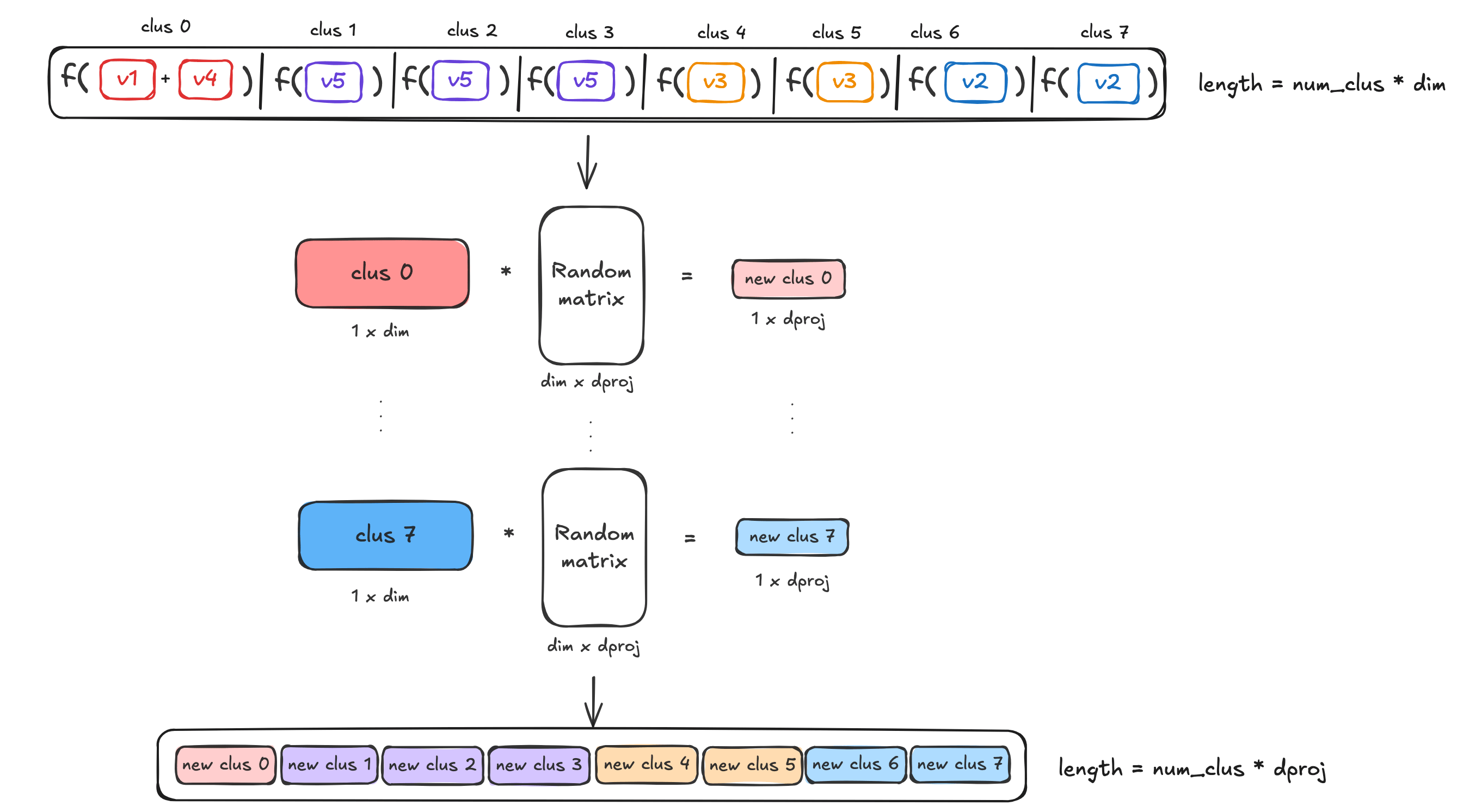
Dimensionality reduction​

To reduce the dependency from the dimensionality of the token embeddings the next step is to reduce the dimensionality. This helps to manage the length of the final encoded vector by applying a random linear projection to make the resulting sub-vectors dkd_kdk​ smaller.

Given the parameter dprojd_{proj}dproj​ we create a random matrix Sdproj×dimS^{d_{proj} \times dim}Sdproj​×dim with ±1\pm1±1 which is used to reduce the dimensionality of each sub-vector.

For each dkd_kdk​ we compute a matrix-vector multiplication:

ψ(dk)=1dproj⋅S⋅dk\psi(d_k)=\frac{1}{\sqrt{d_{proj}}} \cdot S \cdot d_kψ(dk​)=dproj​​1​⋅S⋅dk​

The resulting sub-vector will have length dprojd_{proj}dproj​.

Now the FDE vector will become:

dsingle=(ψ(d1),ψ(d2),…,ψ(dB))d_{single}=(\psi(d_1), \psi(d_2),\dots,\psi(d_B))dsingle​=(ψ(d1​),ψ(d2​),…,ψ(dB​))

Notice the dimensionality will no longer be B∗dimB*dimB∗dim, but B∗dprojB *d_{proj}B∗dproj​ where dproj<<dimd_{proj} << dimdproj​<<dim.

MUVERA steps 3

Applying a random projection may seem... random! However, this is part of the secret sauce of making MUVERA work. The original authors chose the particular distribution of the random matrics to follow the Johnson Lindenstrauss Lemma, which in turn preserves the dot products between vectors that we care about.

Multiple Repetitions​

To increase the accuracy coming from the approximation steps, we can repeat the processes above (space partitioning + dimensionality reduction) multiple times concatenating all vectors together.

Suppose we repeat the partition and dim reduction steps RrepsR_{reps}Rreps​ times obtaining different single-vector we can concatenate them obtaining only one single-vector.

dsingle=(dsingle1,dsingle2,…,dsingleRreps)d_{single}=(d_{single_1}, d_{single_2}, \dots, d_{single_{R_{reps}}} )dsingle​=(dsingle1​​,dsingle2​​,…,dsingleRreps​​​)

The resulting vector will have dimensionality Rreps∗B∗dprojR_{reps}*B*d_{proj}Rreps​∗B∗dproj​ .

Final Projection​

The vector obtained concatenating all the single vectors could lead to quite long vectors. In order to reduce its dimensionality we can apply a final random projection the same described in step 2 to the overall vector. Using the random matrix Sdfinal×dimS^{d_{final} \times dim}Sdfinal​×dim where dfinald_{final}dfinal​ is a parameter

FDE(D)=ψfinal(dsingle)FDE(D)=\psi_{final}(d_{single})FDE(D)=ψfinal​(dsingle​)

This will reduce the final FDE dimensionality yet again.

MUVERA parameters​

During the description of the algorithm we have seen four parameters:

• ksimk_{sim}ksim​: number of Gaussian vectors sampled, the number of buckets we will have is B=2ksimB=2^{k_{sim}}B=2ksim​
• dprojd_{proj}dproj​: dimensionality of the sub-vectors representing a bucket in the space
• RrepsR_{reps}Rreps​: number of times the partition step and dimensionality step are executed
• dfinald_{final}dfinal​: final dimensionality of the FDE vector - FDE(D)∈RdfinalFDE(D)\in\mathbb{R}^{d_{final}}FDE(D)∈Rdfinal​

At the end of the day, these are the key tunable parameters from the user perspective. In terms of the Weaviate implementation - we've chosen what we see as sensible defaults for the majority of use cases.

But as always, you can tune these to suit your particular needs. But before you do that - here's some real-life results from our internal testing.

Impact of MUVERA​

So what are the effects of MUVERA? As in - what's in it for you?

To evaluate this, we used the LoTTE benchmark, in particular lotte-lifestyle which is made up of around 119k documents. Each document was encoded using colbertv2.0 which produced an average of 130 vectors per document.

This would produce 15M vectors of dimensionality 128. This means the total number of floating points stored would be 1.9B, leading to around 8 GB of memory. It might seem that extreme, until you realize that this is a small-ish dataset - and that's even before we add the HNSW graph itself!

On the other hand, if we enable MUVERA with the following parameters:

• ksim=4k_{sim}=4ksim​=4
• dproj=16d_{proj}=16dproj​=16
• Rreps=10R_{reps}=10Rreps​=10

We would encode each document using one vector of dimensionality 2560 = 2^4*16*10 , ending up with 304M floating points stored. An instant saving of almost 80% in memory footprint.

In addition to this, when enabling MUVERA we would have a HNSW (Hierarchical Navigable Small World Graph) with 119k nodes whereas without it, the graph would have 15M nodes, each node having many (e.g. 32-128) edges to other nodes. At a maxConnections value of 128, for example, this could save tens of gigabytes of memory.

Take a look at the example outputs below from our experimentation. We compare four scenarios:

• Raw multi-vector embeddings + SQ
• MUVERA with scalar quantization (SQ)

Heap allocation without using MUVERA + sq vs. MUVERA + sq

Import time without using MUVERA + sq vs. MUVERA + sq

QPS without using MUVERA + sq vs. MUVERA + sq

Recall without using MUVERA + sq vs. MUVERA + sq

As expected, there is a significant reduction in memory footprint, going from a baseline of around 12 GB to under 1GB for MUVERA.

What does that mean in terms of dollar amounts? Well, the difference in compute costs at a hyperscaler for a server with 12 GB of memory and another with 1 GB would be many tens of thousands of dollars per year, if not hundreds of thousands.

If your dataset size ranges in tens or millions or more, as many of our users' datasets do, this may already be a strong motivator for MUVERA.

Not only that, the time taken to import the data is hugely different here. By that, we refer to the time taken for the object data to be added to Weaviate, and the vectors added to the HNSW index. Since adding multi-vector embedding requires tens or hundreds of vectors to be added to the index, this adds significant overhead.

With MUVERA, this is reduced significantly once again. Adding the ~110k objects in the LoTTE dataset required over 20 minutes (or, only around 100 objects/s) in the baseline case, but it was down to around 3-6 minutes in the various MUVERA scenarios.

Again, when considering working at scale - you may want to consider a ~3 hour job to import a million objects may be viable for you. If not, that may be another strong incentive for you to consider MUVERA.

It should be noted that at the same ef value, enabling MUVERA increases query throughput as well, owing to only needing to deal with one vector per object rather than multiple. But - that's not quite an apples-to-apples comparison. And here's why.

Costs: Recall & query throughput​

As we can see in the charts, the main drawback of MUVERA is a loss on the recall side. The downside also may seem particularly challenging, since multi-vector models achieve such high recall values in the first place.

However, some of this can be mitigated through the HNSW search settings. As the graphs show, setting a higher ef value in the query settings (e.g. >512) can increase recall to 80%+, and over 90% at 2048.

As ef increases the retrieved candidate set, it does have a knock-on effect of decreasing the query throughput (measured by queries per second, or qps).

In other words - the main tradeoffs of enabling MUVERA are going to be the reduction in recall, and associated reduction in throughput by needing to use higher ef values.

Nothing's ever so simple, right? 😅 What's clear from these charts is that there is a definite case to be made for using MUVERA. The specifics, however, would very much depend on your priorities.

Wrap-up​

MUVERA compared

In summary, MUVERA offers a compelling path forward for working with multi-vector models at scale.

By transforming multi-vector representations into fixed dimensional encodings, it delivers significant memory savings and improved query speeds while maintaining relatively strong retrieval quality.

Weaviate's implementation of MUVERA enables the ability to further compress these encodings with quantization for production deployments at scale, dramatically reducing the cost and overhead needed for multi-vector embeddings.

As always - using the Weaviate implementation (available form Weaviate 1.31 onwards) may be the easiest part of all this. You may be surprised to hear that just a couple of lines of code is all you need to enable MUVERA in a Weaviate collection.

If your use case could benefit from using multi-vector embeddings, and your use case may require a non-trivial dataset size, MUVERA could be a part of the solution set for you. We encourage you to check it out.

Ready to start building?​

Check out the Quickstart tutorial, or build amazing apps with a free trial of Weaviate Cloud (WCD).