Interactive Image Segmentation with Graph-Cut in Python
In this article, interactive image segmentation with graph-cut is going to be discussed. and it will be used to segment the source object from the background in an image. This segmentation technique was proposed by Boycov and Jolli in this paper. This problem appeared as a homework assignment here., and also in this lecture video from the Coursera image processing course by Duke university.
Problem Statement: Interactive graph-cut segmentation
Let’s implement “intelligent paint” interactive segmentation tool using graph cuts algorithm on a weighted image grid. Our task will be to separate the foreground object from the background in an image.
Since it can be difficult sometimes to automatically define what’s foreground and what’s background for an image, the user is going to help us with a few interactive scribble lines using which our algorithm is going to identify the foreground and the background, after that it will be the algorithms job to obtain a complete segmentation of the foreground from the background image.
The following figures show how an input image gets scribbling from a user with two different colors (which is also going to be input to our algorithm) and the ideal segmented image output.
Scribbled Input Image Expected Segmented Output Image 
The Graph-Cut Algorithm
The following describes how the segmentation problem is transformed into a graph-cut problem:
-
Let’s first define the Directed Graph G = (V, E) as follows:
- Each of the pixels in the image is going to be a vertex in the graph. There will be another couple of special terminal vertices: a source vertex (corresponds to the foreground object) and a sink vertex (corresponds to the background object in the image). Hence, |V(G)| = width x height + 2.
- Next, let’s defines the edges of the graph. As obvious, there is going to be two types of edges: terminal (edges that connect the terminal nodes to the non-terminal nodes) and non-terminal (edges that connect the non-terminal nodes only).
- There will be a directed edge from the terminal node source to each of non-terminal nodes in the graph. Similarly, a directed edge will be there from each non-terminal node (pixel) to the other terminal node sink. These are going to be all the terminal edges and hence, |**E_T(G)**| = 2 x width x height.
- Each of the non-terminal nodes (pixels) are going to be connected by edges with the nodes corresponding to the neighboring pixels (defined by 4 or 8 neighborhood of a pixel). Hence, |E_N(G)| = |**Nb**d| x width x height.
-
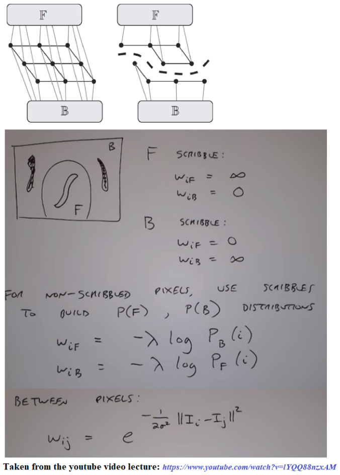
Now let’s describe how to compute the edge weights in this graph.
-
In order to compute the terminal edge weights, we need to estimate the feature distributions first, i.e., starting with the assumption that each of the nodes corresponding to the scribbled pixels have the probability 1.0 (since we want the solution to respect the regional hard constraints marked by the user-seeds / scribbles) to be in foreground or background object in the image (distinguished by the scribble color, e.g.), we have to compute the probability that a node belongs to the foreground (or background) for all the other non-terminal nodes.
-
The simplest way to compute
 and
and  is to first fit a couple of Gaussian distributions on the scribbles by computing the parameters (μ, ∑)
with MLE from the scribbled pixel intensities and then computing the (class-conditional) probabilities from the individual pdfs (followed by a normalization) for each of the pixels as shown in the next figures. The following code fragment show how the pdfs are being computed.import numpy as np from collections import defaultdict
def compute_pdfs(imfile, imfile_scrib): '''
# Compute foreground and background pdfs # input image and the image with user scribbles ''' rgb = mpimg.imread(imfile)\[:,:,:3\] yuv = rgb2yiq(rgb) rgb\_s = mpimg.imread(imfile\_scrib)\[:,:,:3\] yuv\_s = rgb2yiq(rgb\_s) # find the scribble pixels scribbles = find\_marked\_locations(rgb, rgb\_s) imageo = np.zeros(yuv.shape) # separately store background and foreground scribble pixels in the dictionary comps comps = defaultdict(lambda:np.array(\[\]).reshape(0,3)) for (i, j) in scribbles: imageo\[i,j,:\] = rgbs\[i,j,:\] # scribble color as key of comps comps\[tuple(imageo\[i,j,:\])\] = np.vstack(\[comps\[tuple(imageo\[i,j,:\])\], yuv\[i,j,:\]\]) mu, Sigma = {}, {} # compute MLE parameters for Gaussians for c in comps: mu\[c\] = np.mean(comps\[c\], axis=0) Sigma\[c\] = np.cov(comps\[c\].T) return (mu, Sigma)- In order to compute the non-terminal edge weights, we need to compute the similarities in between a pixel node and the nodes corresponding to its neighborhood pixels, e.g., with the formula shown in the next figures (e.g., how similar neighborhood pixels are in RGB / YIQ space).
-
-
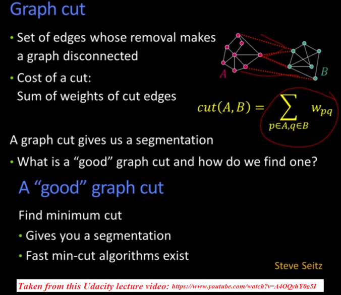
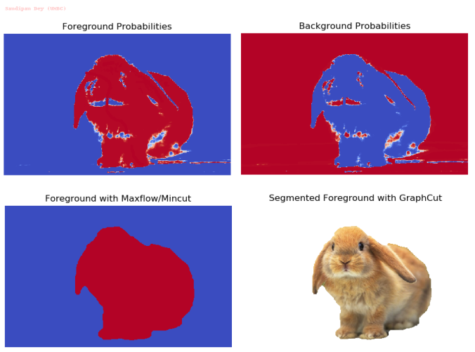
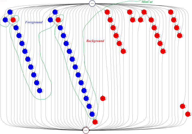
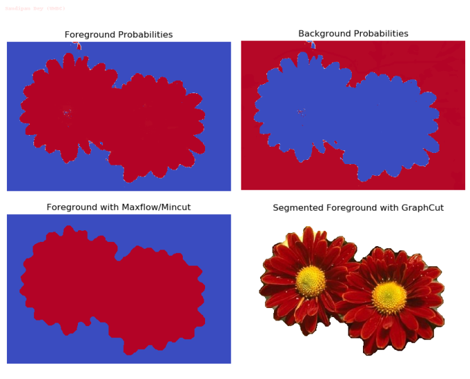
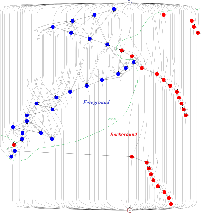
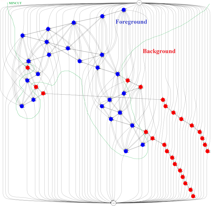
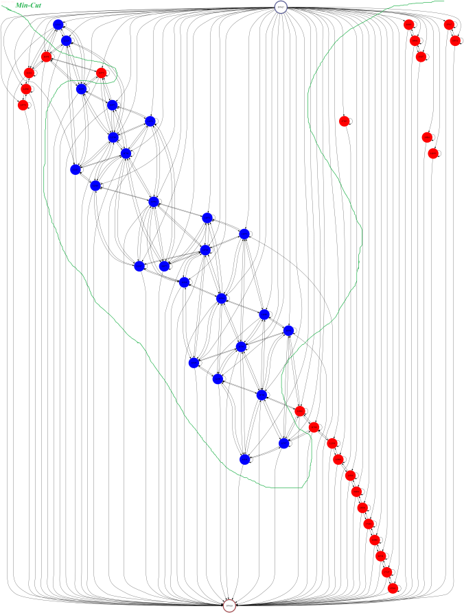
Now that the underlying graph is defined, the segmentation of the foreground from the background image boils down to computing the min-cut in the graph or equivalently computing the max-flow (the dual problem) from the source to sink.
-
The intuition is that the min-cut solution will keep the pixels with high probabilities to belong to the side of the source (foreground) node and likewise the background pixels on the other side of the cut near the sink (background) node, since it’s going to respect the (relatively) high-weight edges (by not going through the highly-similar pixels).
-
There are several standard algorithms, e.g., Ford-Fulkerson (by finding an augmenting path with O(E max| f |) time complexity) or Edmonds-Karp (by using bfs to find the shortest augmenting path, with O(VE2) time complexity) to solve the max-flow problem, typical implementations of these algorithms run pretty fast, in polynomial time in V, E. Here we are going to use a different implementation (with pymaxflow) based on Vladimir Kolmogorov, which is shown to run faster on many images empirically in this paper.


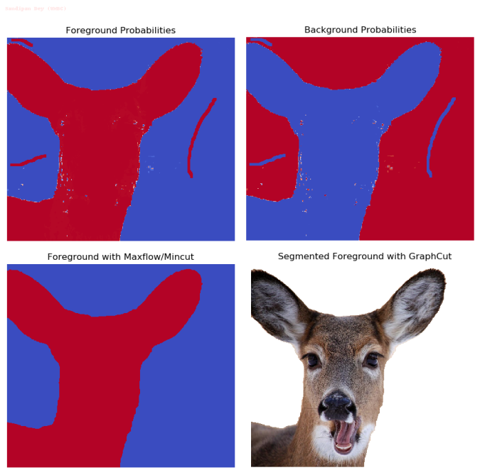
Results
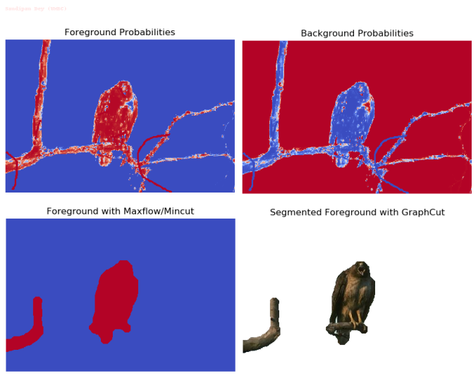
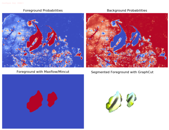
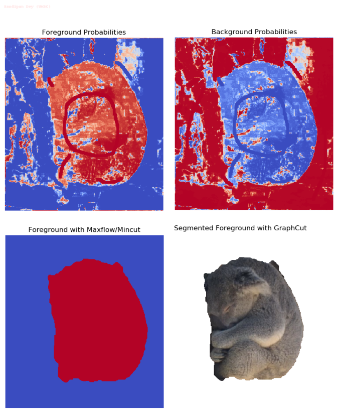
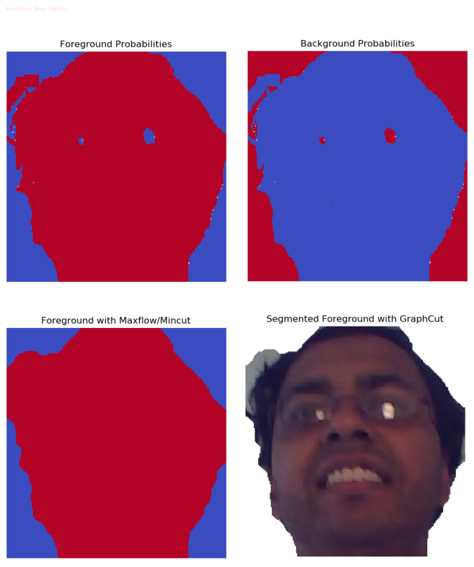
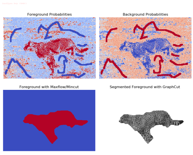
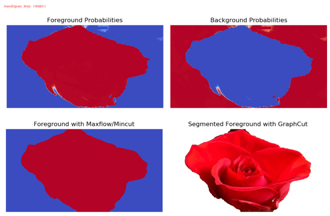
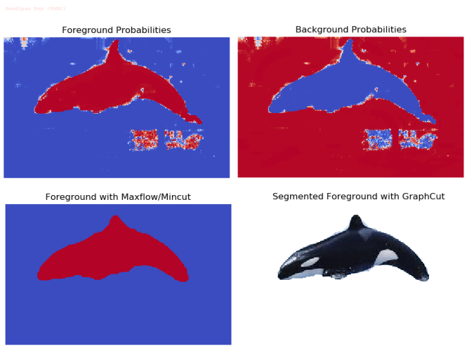
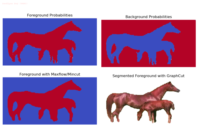
The following figures / animations show the interactive-segmentation results (computed probability densities, subset of the flow-graph & min-cut, final segmented image) on a few images, some of them taken from the above-mentioned courses / videos, some of them taken from Berkeley Vision dataset.
Input Image
Input Image with Scribbles
Fitted Densities from Color Scribbles

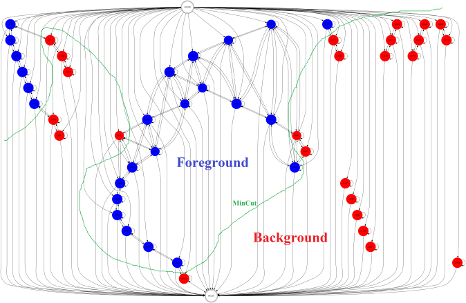
A Tiny Sub-graph with Min-Cut
**Input Image
**
Input Image with Scribbles
Fitted Densities from Color Scribbles

A Tiny Sub-graph with Min-Cut 
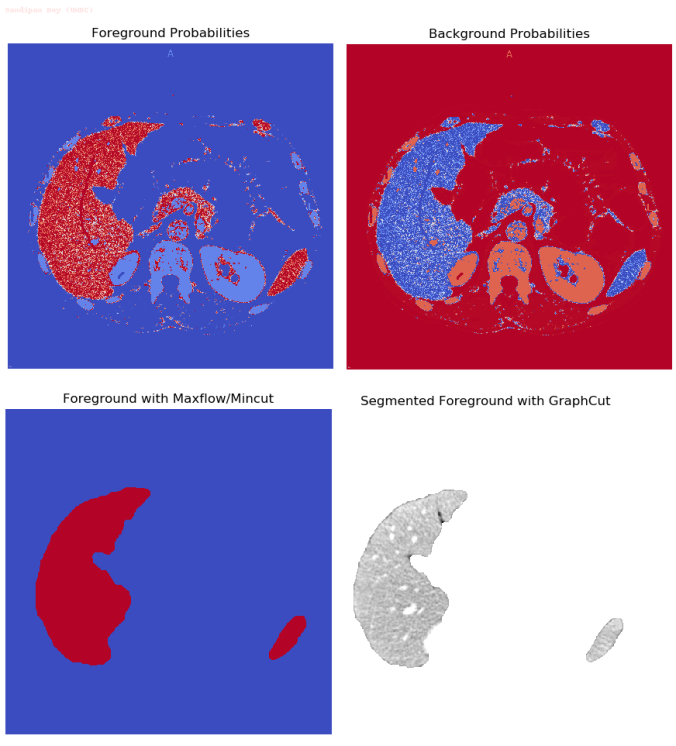
Input Image (liver)

Input Image with Scribbles
Fitted Densities from Color Scribbles

Input Image
Input Image with Scribbles

Fitted Densities from Color Scribbles
**
**
A Tiny Sub-graph of the flow-graph with Min-Cut

Input Image

Input Image with Scribbles
Input Image
Input Image with Scribbles
Fitted Densities from Color Scribbles


A Tiny Sub-graph of the flow-graph with Min-Cut
**Input Image
**
Input Image with Scribbles

A Tiny Sub-graph of the flow-graph with Min-Cut
Input Image Input Image with Scribbles


Input Image
Input Image with Scribbles
A Tiny Sub-graph of the flow-graph with Min-Cut
Input Image
Input Image with Scribbles

**Fitted Densities from Color Scribbles

**
Input Image

Input Image with Scribbles
Fitted Densities from Color Scribbles
A Tiny Sub-graph of the flow-graph with Min-Cut

Input Image (UMBC Campus Map)
Input Image with Scribbles

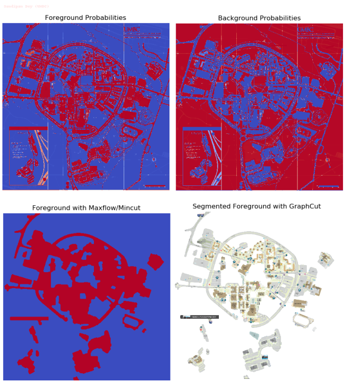
Input Image
Input Image with Scribbles

A Tiny Sub-graph of the flow-graph with Min-Cut (with blue foreground nodes)
Changing the background of an image (obtained using graph-cut segmentation) with another image’s background with cut & paste
The following figures / animation show how the background of a given image can be replaced by a new image using cut & paste (by replacing the corresponding pixels in the new image corresponding to foreground), once the foreground in the original image gets identified after segmentation.
Original Input Image
New Background

